Conducting cylinder
Storyboard 
Variables
Calculations
Calculations
Equations
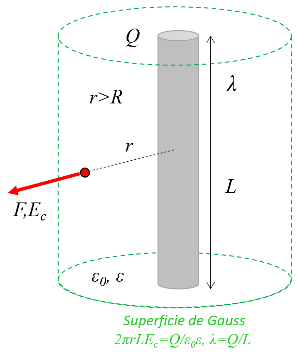
In the case of a cylindrical Gaussian surface, the electric field ($\vec{E}$) is constant in the direction of the versor normal to the section ($\hat{n}$). Therefore, using the variables the charge ($Q$), the electric field constant ($\epsilon_0$), and the dielectric constant ($\epsilon$), the integral over the surface where the electric field is constant ($dS$) can be calculated through the following equation:
For a cylinder characterized by the axle distance ($r$) and the conductor length ($L$), the following applies:
Furthermore, the linear charge density ($\lambda$) is calculated using the charge ($Q$) according to the equation:
Thus, it is established that the electric field, infinite conducting cylinder ($E_c$) is:
The reference electrical, infinite conducting cylinder ($\varphi_c$) is derived from the radial integration of the electric field, infinite conducting cylinder ($E_c$) from the cylinder radius ($r_0$) to the axle distance ($r$), resulting in the following equation:
Furthermore, for the variables the charge ($Q$), the dielectric constant ($\epsilon$), and the electric field constant ($\epsilon_0$), the value of the electric field, infinite conducting cylinder ($E_c$) is given as:
This implies that by performing the integration
$\varphi_c = -\displaystyle\int_{r_0}^r du \displaystyle\frac{ \lambda }{ 2 \pi \epsilon_0 \epsilon u }= -\displaystyle\frac{ \lambda }{ 2 \pi \epsilon_0 \epsilon } \ln\left(\displaystyle\frac{ r }{ r_0 }\right)$
the following equation is obtained:
Examples
In the case of a cylindrical Gaussian surface, the electric field ($\vec{E}$) is constant in the direction of the versor normal to the section ($\hat{n}$). Therefore, using the variables the charge ($Q$), the electric field constant ($\epsilon_0$), and the dielectric constant ($\epsilon$), the integral over the surface where the electric field is constant ($dS$) can be calculated through the following equation:
For a cylinder characterized by the axle distance ($r$) and the conductor length ($L$), the following applies:
what is shown in the graph
Furthermore, the linear charge density ($\lambda$) is calculated using the charge ($Q$) according to the equation:
Thus, it is established that the electric field, infinite conducting cylinder ($E_c$) is:
In the case of a cylindrical Gaussian surface, the electric field ($\vec{E}$) is constant in the direction of the versor normal to the section ($\hat{n}$). Therefore, using the variables the charge ($Q$), the electric field constant ($\epsilon_0$), and the dielectric constant ($\epsilon$), the integral over the surface where the electric field is constant ($dS$) can be calculated through the following equation:
For a cylinder characterized by the axle distance ($r$) and the conductor length ($L$), the following applies:
Furthermore, the linear charge density ($\lambda$) is calculated using the charge ($Q$) according to the equation:
Thus, it is established that the electric field, infinite conducting cylinder ($E_c$) is:
As illustrated in the following graph:
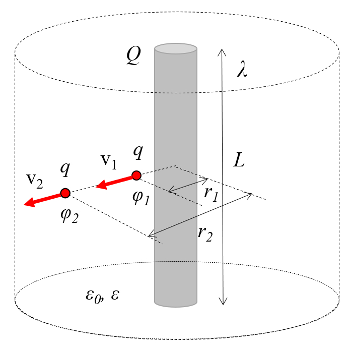
the field at two points must have the same energy. Therefore, the variables the charge ($Q$), the particle mass ($m$), the speed 1 ($v_1$), the speed 2 ($v_2$), and the electric potential 1 ($\varphi_1$) according to the equation:
and the electric potential 2 ($\varphi_2$), according to the equation:
must satisfy the following relationship:
The linear charge density ($\lambda$) is calculated as the charge ($Q$) divided by the conductor length ($L$):
The electric field, infinite conducting cylinder ($E_c$) is with the pi ($\pi$), the electric field constant ($\epsilon_0$), the dielectric constant ($\epsilon$), the linear charge density ($\lambda$) and the axle distance ($r$) is equal to:
The electric field, infinite conducting cylinder ($E_c$) is with the pi ($\pi$), the electric field constant ($\epsilon_0$), the dielectric constant ($\epsilon$), the linear charge density ($\lambda$) and the axle distance ($r$) is equal to:
The reference electrical, infinite conducting cylinder ($\varphi_c$) is with the pi ($\pi$), the electric field constant ($\epsilon_0$), the dielectric constant ($\epsilon$), the linear charge density ($\lambda$), the axle distance ($r$) and the cylinder radius ($r_0$) is equal to:
The reference electrical, infinite conducting cylinder ($\varphi_c$) is with the pi ($\pi$), the electric field constant ($\epsilon_0$), the dielectric constant ($\epsilon$), the linear charge density ($\lambda$), the axle distance ($r$) and the cylinder radius ($r_0$) is equal to:
Electric potentials, which represent potential energy per unit of charge, influence how the velocity of a particle varies. Consequently, due to the conservation of energy between two points, it follows that in the presence of variables the charge ($q$), the particle mass ($m$), the speed 1 ($v_1$), the speed 2 ($v_2$), the electric potential 1 ($\varphi_1$), and the electric potential 2 ($\varphi_2$), the following relationship must be satisfied:
ID:(2075, 0)