
Examples of electrical potentials
Storyboard 
With the examples of the electric fields calculated above, the electric potentials are calculated.
ID:(1562, 0)
Conductor sphere with charge
Definition
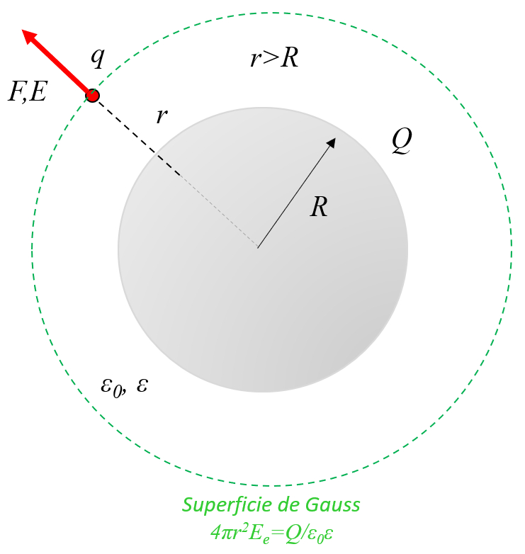
In a conducting sphere with charges, these are distributed on the surface and with it the field inside is null. Outside it behaves like a point charge that is in the center of the sphere:
ID:(11451, 0)
Insulating sphere with homogeneous charge
Image
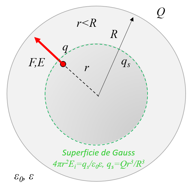
An insulating sphere in which charges have been homogeneously distributed, which cannot be moved because it is an insulating material, has an electric field that grows linearly inside and decreases with the inverse of the radius squared:
ID:(11450, 0)
Loaded infinite wire or cylinder, in vacuum
Note
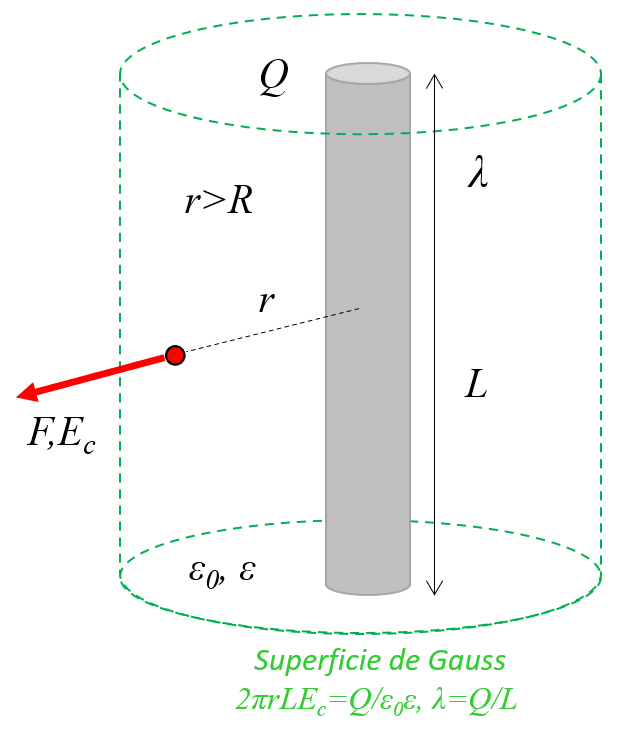
In a conductor wire or cylinder with charges, these are distributed throughout the object, behaving like a long chain of point loads aligned on the axis:
ID:(11452, 0)
Infinite conductor plane with load
Quote
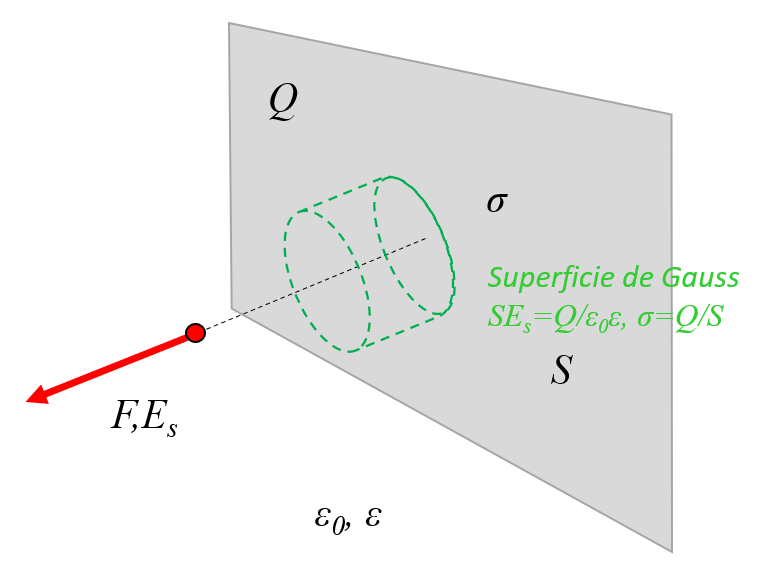
In a conducting plane, a Gaussian surface can be defined as a cylinder. Since the lateral walls are orthogonal to the electric field, they do not contribute to the net flux. Therefore, the only parts that contribute are the cylinder's end caps, which are surfaces parallel to the plane:
ID:(11453, 0)
Simple model for two plates with opposite charges
Exercise
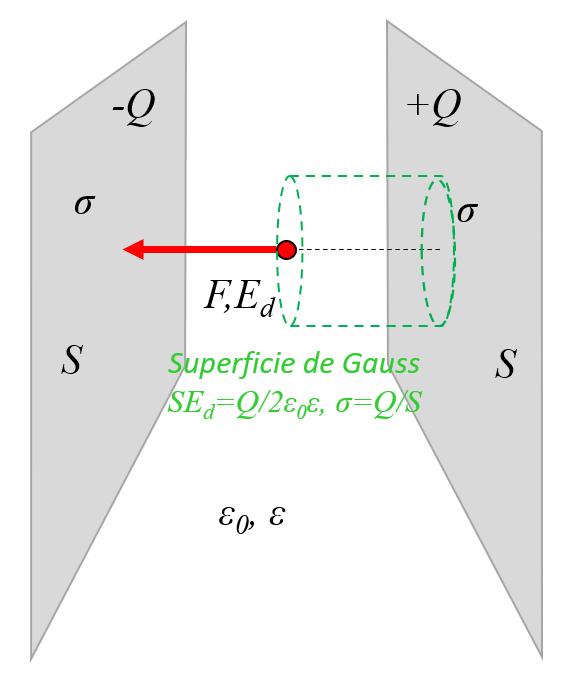
To be able to calculate the field between the two plates in a simple way, it can be assumed that the external field is compensated and that most of it is only between the plates:
ID:(11455, 0)
Examples of electrical potentials
Description
With the examples of the electric fields calculated above, the electric potentials are calculated.
Variables
Calculations
Calculations
Equations
The electric potential, point charge ($\varphi_p$) is calculated from the radial integration of the electric field of a point charge ($E_p$) from the radius ($r$) to infinity, which results in
| $ \varphi_p = -\displaystyle\int_r^{\infty} du\,E_p$ |
On the other hand, for the charge ($Q$), the dielectric constant ($\epsilon$), and the electric field constant ($\epsilon_0$), the value of the electric field of a point charge ($E_p$) is
| $ E_p =\displaystyle\frac{1}{4 \pi \epsilon_0 \epsilon }\displaystyle\frac{Q}{ r ^2}$ |
This implies that by integrating
$\varphi_p = -\displaystyle\int_{r}^{\infty} du \displaystyle\frac{ Q }{4 \pi \epsilon_0 \epsilon u^2 }= -\displaystyle\frac{ Q }{ 4 \pi \epsilon_0 \epsilon }\displaystyle\frac{1}{ r }$
we obtain
| $ \varphi_p = -\displaystyle\frac{ Q }{4 \pi \epsilon_0 \epsilon }\displaystyle\frac{1}{ r } $ |
(ID 11576)
As the potential difference is the reference electrical, insulating sphere, inner ($\varphi_i$) with the electric field, sphere, interior ($E_i$) and the radius ($r$), we get:
| $ \varphi_i = -\displaystyle\int_0^ r du\, E_i $ |
Given that the electric field, sphere, interior ($E_i$) with the pi ($\pi$), the charge ($Q$), the electric field constant ($\epsilon_0$), the dielectric constant ($\epsilon$), the sphere radius ($R$), and the distance between charges ($r$) is equal to:
| $ E_i =\displaystyle\frac{1}{4 \pi \epsilon_0 \epsilon }\displaystyle\frac{ Q r }{ R ^3 }$ |
In spherical coordinates, this is:
$\varphi_i = -\displaystyle\int_0^{r} du \displaystyle\frac{ Q u }{4 \pi \epsilon_0 \epsilon R ^3 }= -\displaystyle\frac{ Q }{ 8 \pi \epsilon_0 \epsilon }\displaystyle\frac{ r ^2 }{ R ^3 }$
Therefore, the reference electrical, insulating sphere, inner ($\varphi_i$) with the distance between charges ($r$) results in:
| $ \varphi_i = -\displaystyle\frac{ Q }{8 \pi \epsilon_0 \epsilon }\displaystyle\frac{ r ^2 }{ R ^3 }$ |
(ID 11583)
As the potential difference is the reference electrical, sphere, outer ($\varphi_e$) with the electric field, sphere, outer ($E_e$), the electric field, sphere, interior ($E_i$), the sphere radius ($R$), and the radius ($r$), we get:
| $ \varphi_e = - \displaystyle\int_0^ R du\, E_i - \displaystyle\int_ R ^ r du\, E_e $ |
Given that the electric field, sphere, outer ($E_e$) with the pi ($\pi$), the charge ($Q$), the electric field constant ($\epsilon_0$), the dielectric constant ($\epsilon$), and the distance between charges ($r$) is equal to:
| $ E_e=\displaystyle\frac{1}{4 \pi \epsilon_0 \epsilon }\displaystyle\frac{ Q }{ r ^2 }$ |
and that the electric field, sphere, interior ($E_i$) with the internal radius ($r_i$) is equal to:
| $ E_i =\displaystyle\frac{1}{4 \pi \epsilon_0 \epsilon }\displaystyle\frac{ Q r }{ R ^3 }$ |
In spherical coordinates, we have:
$\varphi_e = -\displaystyle\int_0^R du \displaystyle\frac{ Q u }{4 \pi \epsilon_0 \epsilon R ^3 } -\displaystyle\int_R^r du \displaystyle\frac{ Q }{4 \pi \epsilon_0 \epsilon u ^2 }= -\displaystyle\frac{ 1 }{ 4 \pi \epsilon_0 \epsilon }\displaystyle\frac{ Q }{ r }$
Therefore, the reference electrical, sphere, outer ($\varphi_e$) results in:
| $ \varphi_e = -\displaystyle\frac{ 1 }{4 \pi \epsilon_0 \epsilon }\displaystyle\frac{ Q }{ r } $ |
(ID 11584)
The reference electrical, infinite conducting cylinder ($\varphi_c$) is derived from the radial integration of the electric field, infinite conducting cylinder ($E_c$) from the cylinder radius ($r_0$) to the axle distance ($r$), resulting in the following equation:
| $ \varphi_c = -\displaystyle\int_{r_0}^r du E_c$ |
Furthermore, for the variables the charge ($Q$), the dielectric constant ($\epsilon$), and the electric field constant ($\epsilon_0$), the value of the electric field, infinite conducting cylinder ($E_c$) is given as:
| $ E_c =\displaystyle\frac{1}{2 \pi \epsilon_0 \epsilon }\displaystyle\frac{ \lambda }{ r }$ |
This implies that by performing the integration
$\varphi_c = -\displaystyle\int_{r_0}^r du \displaystyle\frac{ \lambda }{ 2 \pi \epsilon_0 \epsilon u }= -\displaystyle\frac{ \lambda }{ 2 \pi \epsilon_0 \epsilon } \ln\left(\displaystyle\frac{ r }{ r_0 }\right)$
the following equation is obtained:
| $ \varphi_c = -\displaystyle\frac{ \lambda }{ 2 \pi \epsilon_0 \epsilon }\ln\left(\displaystyle\frac{ r }{ r_0 }\right)$ |
(ID 11585)
In the case of an infinite plate, the relationship between the electric potential, infinite plate ($\varphi_s$), the electric field of an infinite plate ($E_s$), and the position on the z axis ($z$) is established by the following equation:
| $ \varphi_s = -\displaystyle\int_0^z du\,E_s$ |
Similarly, the relationship involving the electric field of an infinite plate ($E_s$), the electric field constant ($\epsilon_0$), the dielectric constant ($\epsilon$), and the charge density by area ($\sigma$) is defined as:
| $ E_s =\displaystyle\frac{ \sigma }{ 2 \epsilon_0 \epsilon }$ |
In spherical coordinates, this is expressed as:
$\varphi_s = -\displaystyle\int_0^z du \displaystyle\frac{ \sigma }{2 \epsilon_0 \epsilon }= -\displaystyle\frac{ \sigma }{2 \epsilon_0 \epsilon } z$
Finally, the relationship that includes the electric potential, infinite plate ($\varphi_s$) and the position on the z axis ($z$) is determined by the following equation:
| $ \varphi_s = -\displaystyle\frac{ \sigma }{2 \epsilon_0 \epsilon } z $ |
(ID 11586)
The reference electrical, two infinity plates ($\varphi_d$) in relation to the electric field, two infinite plates ($E_d$) and the position on the z axis ($z$) is given by:
| $ \varphi_d = -\displaystyle\int_0^z du\,E_d$ |
Similarly, the electric field, two infinite plates ($E_d$) in relation to the electric field constant ($\epsilon_0$), the dielectric constant ($\epsilon$), and the charge density by area ($\sigma$) is defined by:
| $ E_d =\displaystyle\frac{ \sigma }{ \epsilon_0 \epsilon }$ |
By integrating from the origin, we obtain:
$\varphi_d = -\displaystyle\int_0^z du \displaystyle\frac{ \sigma }{ \epsilon_0 \epsilon }= -\displaystyle\frac{ \sigma }{ \epsilon_0 \epsilon } z$
Thus, the reference electrical, two infinity plates ($\varphi_d$) is given by:
| $ \varphi_d = -\displaystyle\frac{ \sigma }{ \epsilon_0 \epsilon } z $ |
(ID 11587)
Examples
Electric potentials, which represent potential energy per unit of charge, influence how the velocity of a particle varies. Consequently, due to the conservation of energy between two points, it follows that in the presence of variables the charge ($q$), the particle mass ($m$), the speed 1 ($v_1$), the speed 2 ($v_2$), the electric potential 1 ($\varphi_1$), and the electric potential 2 ($\varphi_2$), the following relationship must be satisfied:
| $ \displaystyle\frac{1}{2} m v_1 ^2 + q \varphi_1 = \displaystyle\frac{1}{2} m v_2 ^2 + q \varphi_2 $ |
(ID 11596)
In a conducting sphere with charges, these are distributed on the surface and with it the field inside is null. Outside it behaves like a point charge that is in the center of the sphere:
(ID 11451)
The electric potential, point charge ($\varphi_p$) is with the charge ($Q$), the distance between charges ($r$), the dielectric constant ($\epsilon$) and the electric field constant ($\epsilon_0$) equal to:
| $ \varphi_p = -\displaystyle\frac{ Q }{4 \pi \epsilon_0 \epsilon }\displaystyle\frac{1}{ r } $ |
(ID 11576)
Como la diferencia de potencial con es igual
| $ \varphi_f = -\displaystyle\int_r^{\infty} du\,E_f(u)$ |
con
| $ E_f =\displaystyle\frac{1}{4 \pi \epsilon_0 \epsilon }\displaystyle\frac{Q}{ r ^2}\theta( r - R )$ |
lo que en coordenadas esf ricas es
$\varphi_f = -\displaystyle\int_{\infty}^{r} du \displaystyle\frac{ Q }{4 \pi \epsilon_0 \epsilon u ^2 }= -\displaystyle\frac{ Q }{ 4 \pi \epsilon_0 \epsilon }\displaystyle\frac{1}{ r }$
o sea con
| $ \varphi_f = -\displaystyle\frac{ Q }{4 \pi \epsilon_0 \epsilon }\displaystyle\frac{1}{ r } $ |
(ID 11582)
An insulating sphere in which charges have been homogeneously distributed, which cannot be moved because it is an insulating material, has an electric field that grows linearly inside and decreases with the inverse of the radius squared:
(ID 11450)
The reference electrical, insulating sphere, inner ($\varphi_i$) is with the pi ($\pi$), the charge ($Q$), the electric field constant ($\epsilon_0$), the dielectric constant ($\epsilon$), the distance between charges ($r$) and the sphere radius ($R$) is equal to:
| $ \varphi_i = -\displaystyle\frac{ Q }{8 \pi \epsilon_0 \epsilon }\displaystyle\frac{ r ^2 }{ R ^3 }$ |
(ID 11583)
The reference electrical, sphere, outer ($\varphi_e$) is with the pi ($\pi$), the charge ($Q$), the electric field constant ($\epsilon_0$), the dielectric constant ($\epsilon$) and the distance between charges ($r$) is equal to:
| $ \varphi_e = -\displaystyle\frac{ 1 }{4 \pi \epsilon_0 \epsilon }\displaystyle\frac{ Q }{ r } $ |
(ID 11584)
In a conductor wire or cylinder with charges, these are distributed throughout the object, behaving like a long chain of point loads aligned on the axis:
(ID 11452)
The reference electrical, infinite conducting cylinder ($\varphi_c$) is with the pi ($\pi$), the electric field constant ($\epsilon_0$), the dielectric constant ($\epsilon$), the linear charge density ($\lambda$), the axle distance ($r$) and the cylinder radius ($r_0$) is equal to:
| $ \varphi_c = -\displaystyle\frac{ \lambda }{ 2 \pi \epsilon_0 \epsilon }\ln\left(\displaystyle\frac{ r }{ r_0 }\right)$ |
(ID 11585)
In a conducting plane, a Gaussian surface can be defined as a cylinder. Since the lateral walls are orthogonal to the electric field, they do not contribute to the net flux. Therefore, the only parts that contribute are the cylinder's end caps, which are surfaces parallel to the plane:
(ID 11453)
The electric potential, infinite plate ($\varphi_s$) is with the electric field constant ($\epsilon_0$), the dielectric constant ($\epsilon$), the charge density by area ($\sigma$) and the position on the z axis ($z$) is equal to:
| $ \varphi_s = -\displaystyle\frac{ \sigma }{2 \epsilon_0 \epsilon } z $ |
(ID 11586)
To be able to calculate the field between the two plates in a simple way, it can be assumed that the external field is compensated and that most of it is only between the plates:
(ID 11455)
The reference electrical, two infinity plates ($\varphi_d$) is with the electric field constant ($\epsilon_0$), the dielectric constant ($\epsilon$), the charge density by area ($\sigma$) and the position on the z axis ($z$) is equal to:
| $ \varphi_d = -\displaystyle\frac{ \sigma }{ \epsilon_0 \epsilon } z $ |
(ID 11587)
ID:(1562, 0)