
Heat conduction mechanism
Definition 
The heat conducted by a
and the conductivity
ID:(7718, 0)
Conducción por Suelos
Image
El motor de la conducción de calor es la diferencia de temperatura que existe entre los dos extremos de un cuerpo. Si ambas temperaturas son iguales no existiría flujo de calor.
En el caso de calefacción la diferencia de temperatura entre la del agua del calefactor y la temperatura ambiente interior genera el flujo de calor para calentar la habitación. Para calefacción crital el tubo se encuentra inmerso en un cemento que tiene típicamente una constante de conducción $\lambda$ del orden de $1.5,J/m^2sK$. Adicionalmente puede existir un revestimiento con baldosas, con un $\lambda$ de $1,J/m^2sK$ o parqué con un $\lambda$ de $0.17,J/m^2sK$.
> Diferencia de temperatura necesaria
>
> Si se requiere que atraviesen $40,W/m^2$ y se tiene que el coeficiente de conducción es del orden de $1,J/m^2sK$, siendo el grosor de la pared de $1,cm$ se tiene que se requiere de una diferencia de temperatura de
>
>$\Delta T=\displaystyle\frac{L}{\lambda}\displaystyle\frac{\dot{Q}}{S}=\displaystyle\frac{0.01,m}{1,J/m^2sK}\displaystyle\frac{40,W/m^2}{1\m^2}=0.4,K$
>
>Si el grosor de la pared fuera diez veces mayor o la conductividad un décimo se requiere de una diferencia de cuatro grados.
Cabe hacer notar que la diferencia de temperatura aquí calculado es aquel entre las dos superficies del medio. Como la temperatura aumenta/disminuye dentro del medio liquido/gaseoso en contacto, la diferencia total entre ambos medios es mayor a la entre ambas caras del conductor.
ID:(7731, 0)
Heat transport
Note
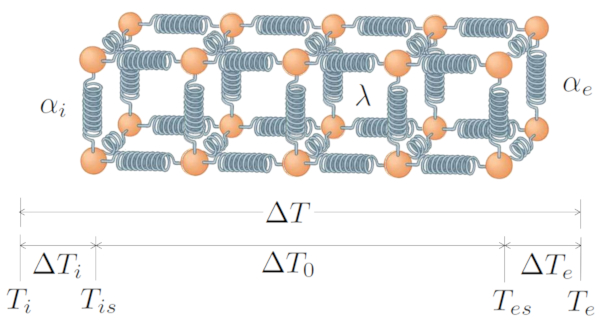
The basic system includes a transfer generated by the temperature difference ($\Delta T$), which consists of the temperature difference at internal interface ($\Delta T_i$), the temperature difference in the conductor ($\Delta T_0$), and the temperature difference at external interface ($\Delta T_e$). Therefore:
| $ \Delta T = \Delta T_i + \Delta T_0 + \Delta T_e $ |
With the heat flow rate ($q$) being responsible for the transfer between the interior and the conductor, using the internal transmission coefficient ($\alpha_i$):
| $ q = \alpha_i \Delta T_i $ |
Conduction involves the thermal conductivity ($\lambda$) and the conductor length ($L$):
| $ q = \displaystyle\frac{ \lambda }{ L } \Delta T_0 $ |
And the transfer from the conductor to the exterior, with the external transmission coefficient ($\alpha_e$), is represented by:
| $ q = \alpha_e \Delta T_e $ |
All this is graphically represented by:
ID:(7723, 0)
Total heat flow transportation
Quote
When the material includes multiple conductors connected in series, the total transport coefficient (multiple medium, two interfaces) ($k$) is calculated from the external transmission coefficient ($\alpha_e$), the internal transmission coefficient ($\alpha_i$), the thermal conductivity element i ($\lambda_i$), and the element length i ($L_i$) using the equation:
| $\displaystyle\frac{1}{ k }=\displaystyle\frac{1}{ \alpha_i }+\displaystyle\frac{1}{ \alpha_e }+\sum_i\displaystyle\frac{ L_i }{ \lambda_i }$ |
This process is illustrated in the following diagram:
![]()
ID:(7721, 0)
Temperature Profile
Exercise
Typically, the temperature variation within a conductor follows a linear pattern. However, in the case of gaseous and/or liquid media in contact with the conductor, there is a gradual temperature variation from the center of the medium to the surface, as depicted in the following image:
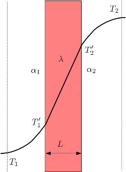
the outer surface temperature ($T_{es}$) depends on the outdoor Temperature ($T_e$), the coefficient of total transportation ($k$), the external transmission coefficient ($\alpha_e$), and the temperature difference ($\Delta T$):
| $ T_{es} = T_e + \displaystyle\frac{ k }{ \alpha_e } \Delta T $ |
the inner surface temperature ($T_{is}$) is a function of the indoor temperature ($T_i$) and the internal transmission coefficient ($\alpha_i$):
| $ T_{is} = T_i - \displaystyle\frac{ k }{ \alpha_i } \Delta T $ |
and the temperature difference ($\Delta T$):
| $ \Delta T = T_i - T_e $ |
ID:(7722, 0)
Coeficiente de Transporte
Equation
En el caso de la calefacción crital uno de los sistemas es agua y el otro aire. En el caso del agua los flujos $J$ típicos son del orden de 100 l/h. Si el tubo tiene un radio $R$ de 8 mm esto significa que la velocidad del agua $v$ se puede calcular de
$J=Sv=\pi R^2v$
donde $S$ es la sección del tubo. Por ello en el caso de la calefacción crital la velocidad típica es del orden de 0.13 m/s. Con ello el coeficiente de transmisión del agua-suelo es del orden de 1075 J/m2sK.
En el caso del aire la velocidad es del orden de cero y con ello el coeficiente de transmisión del orden de 5.4 J/m2sK.
Por ultimo el cemento presenta un coeficiente de 2.3 J/msK. Si la distancia entre tubo y superficie es del orden de 1 cm se tiene que el coeficiente de transporte $k$ es del orden de 5.4 J/m2sK.
ID:(7725, 0)
Heat Transport Simulator
Script
The heat transport simulator through a wall allows estimating the key parameters and plotting the temperature profile along the system.
There are three ways to use the simulator:
• Calculate the heat transport constant $k$ and the achieved power density $\dot{Q}$ given temperatures, thermal conductivities $\lambda_i$, layer widths $L_i$, and transfer constant $\alpha$. In this case, select the line for the heat transport constant and power density to recalculate and overwrite these values.
• Calculate the width of one of the layers based on its thermal conductivity, along with other geometric and material parameters of the system, and either the heat transport constant $k$ or the power density $\dot{Q}$. In this case, choose the line corresponding to the layer you want to calculate and leave the thermal conductivity field empty.
• Calculate the thermal conductivity of one of the layers based on its width, along with other geometric and material parameters of the system, and either the heat transport constant $k$ or the power density $\dot{Q}$. In this case, choose the line corresponding to the layer you want to calculate and leave the width field empty.
If the external system corresponds to a different material, such as soil instead of air, leave the transfer coefficient field empty.
ID:(7736, 0)
Modelo Simplificado
Storyboard
Variables
Calculations
Calculations
Equations
With the temperature difference at internal interface ($\Delta T_i$), the temperature difference in the conductor ($\Delta T_0$), the temperature difference at external interface ($\Delta T_e$), and the temperature difference ($\Delta T$), we obtain
which can be rewritten with the heat transported ($dQ$), the time variation ($dt$), the section ($S$)
and with the thermal conductivity ($\lambda$) and the conductor length ($L$)
and
as
$\Delta T = \Delta T_i + \Delta T_0 + \Delta T_e = \displaystyle\frac{1}{S} \frac{dQ}{dt} \left(\displaystyle\frac{1}{\alpha_i} + \displaystyle\frac{1}{\alpha_e} + \displaystyle\frac{L}{\lambda}\right) = \displaystyle\frac{1}{Sk} \displaystyle\frac{dQ}{dt}$
resulting in
Examples
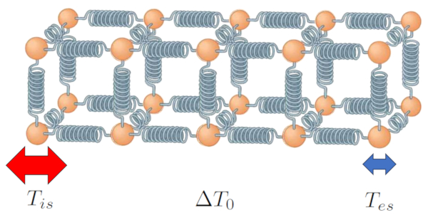
To understand how heat is conducted in a solid or liquid, we can imagine that the material is composed of particles (atoms or molecules) that interact through forces that can be modeled as springs. In this framework, heat is understood as the internal energy of the particles, which manifests itself as oscillations.
When the ends of a body are subjected to different temperatures, the particles at each end vibrate with different amplitudes:
Oscillating particles transmit their motion to their neighbors through the binding forces, propagating the oscillation and the corresponding thermal energy. Over time, the entire chain of particles will oscillate, with larger amplitudes at the hotter end (e.g., the inner surface temperature ($T_{is}$)) and smaller amplitudes at the cooler end (e.g., the outer surface temperature ($T_{es}$)).
In this way, energy and thus heat propagates through the body as a function of the temperature difference in the conductor ($\Delta T_0$), defined by the following equation:
The heat flux ($q$) is a function of the thermal conductivity ($\lambda$), the conductor length ($L$) and the temperature difference in the conductor ($\Delta T_0$):
El motor de la conducci n de calor es la diferencia de temperatura que existe entre los dos extremos de un cuerpo. Si ambas temperaturas son iguales no existir a flujo de calor.
En el caso de calefacci n la diferencia de temperatura entre la del agua del calefactor y la temperatura ambiente interior genera el flujo de calor para calentar la habitaci n. Para calefacci n crital el tubo se encuentra inmerso en un cemento que tiene t picamente una constante de conducci n $\lambda$ del orden de $1.5,J/m^2sK$. Adicionalmente puede existir un revestimiento con baldosas, con un $\lambda$ de $1,J/m^2sK$ o parqu con un $\lambda$ de $0.17,J/m^2sK$.
> Diferencia de temperatura necesaria
>
> Si se requiere que atraviesen $40,W/m^2$ y se tiene que el coeficiente de conducci n es del orden de $1,J/m^2sK$, siendo el grosor de la pared de $1,cm$ se tiene que se requiere de una diferencia de temperatura de
>
>$\Delta T=\displaystyle\frac{L}{\lambda}\displaystyle\frac{\dot{Q}}{S}=\displaystyle\frac{0.01,m}{1,J/m^2sK}\displaystyle\frac{40,W/m^2}{1\m^2}=0.4,K$
>
>Si el grosor de la pared fuera diez veces mayor o la conductividad un d cimo se requiere de una diferencia de cuatro grados.
Cabe hacer notar que la diferencia de temperatura aqu calculado es aquel entre las dos superficies del medio. Como la temperatura aumenta/disminuye dentro del medio liquido/gaseoso en contacto, la diferencia total entre ambos medios es mayor a la entre ambas caras del conductor.
The basic system includes a transfer generated by the temperature difference ($\Delta T$), which consists of the temperature difference at internal interface ($\Delta T_i$), the temperature difference in the conductor ($\Delta T_0$), and the temperature difference at external interface ($\Delta T_e$). Therefore:
With the heat flow rate ($q$) being responsible for the transfer between the interior and the conductor, using the internal transmission coefficient ($\alpha_i$):
Conduction involves the thermal conductivity ($\lambda$) and the conductor length ($L$):
And the transfer from the conductor to the exterior, with the external transmission coefficient ($\alpha_e$), is represented by:
All this is graphically represented by:
If a medium is moving with a constant of the transmission coefficient dependent on the speed ($\alpha_{wv}$), and the mean speed ($v_m$) is equal to
where the transmission coefficient Independent of the speed ($\alpha_{w0}$) represents the case where the medium is not moving, and the factor velocidad del coefiente de transmisión ($v_{w0}$) is the reference velocity.
The thermal transfer constant of the material for the case of a stationary liquid is equal to $340 J/m^2sK$, while the reference velocity is $0.0278 m/s$.
La transferencia del calor en un medio a otro lleva a que una cantidad de calor
donde
La constante de transferencia t rmica del material es del orden de 350 - 10000 J/m2sK. Este valor depende de la velocidad si uno de los medios es liquido y se desplaza.
In the event that a medium moves with a constant value of ERROR:5250.1 and the transmission coefficient in gases, dependent on speed ($\alpha_{gv}$) is equal to
where the transmission coefficient in gases, independent of speed ($\alpha_{g0}$) represents the scenario where the medium does not move, and the transmission coefficient gas velocity factor ($v_{g0}$) is the reference velocity.
The thermal transfer constant for the material in the case of a stationary gas is equal to $5.6 J/m^2sK$, while the reference velocity is $1.41 m/s$.
When the material includes multiple conductors connected in series, the total transport coefficient (multiple medium, two interfaces) ($k$) is calculated from the external transmission coefficient ($\alpha_e$), the internal transmission coefficient ($\alpha_i$), the thermal conductivity element i ($\lambda_i$), and the element length i ($L_i$) using the equation:
This process is illustrated in the following diagram:
In this way, we establish a relationship that allows us to calculate the heat flow rate ($q$) as a function of the total transport coefficient (multiple medium, two interfaces) ($k$), and the temperature difference ($\Delta T$):
The transport constant
The value of the heat flow rate ($q$) in the transport equation is determined using the internal transmission coefficient ($\alpha_i$), the external transmission coefficient ($\alpha_e$), the thermal conductivity element i ($\lambda_i$) and the element length i ($L_i$) as follows:
Typically, the temperature variation within a conductor follows a linear pattern. However, in the case of gaseous and/or liquid media in contact with the conductor, there is a gradual temperature variation from the center of the medium to the surface, as depicted in the following image:
the outer surface temperature ($T_{es}$) depends on the outdoor Temperature ($T_e$), the coefficient of total transportation ($k$), the external transmission coefficient ($\alpha_e$), and the temperature difference ($\Delta T$):
the inner surface temperature ($T_{is}$) is a function of the indoor temperature ($T_i$) and the internal transmission coefficient ($\alpha_i$):
and the temperature difference ($\Delta T$):
En el caso de la calefacci n crital uno de los sistemas es agua y el otro aire. En el caso del agua los flujos $J$ t picos son del orden de 100 l/h. Si el tubo tiene un radio $R$ de 8 mm esto significa que la velocidad del agua $v$ se puede calcular de
$J=Sv=\pi R^2v$
donde $S$ es la secci n del tubo. Por ello en el caso de la calefacci n crital la velocidad t pica es del orden de 0.13 m/s. Con ello el coeficiente de transmisi n del agua-suelo es del orden de 1075 J/m2sK.
En el caso del aire la velocidad es del orden de cero y con ello el coeficiente de transmisi n del orden de 5.4 J/m2sK.
Por ultimo el cemento presenta un coeficiente de 2.3 J/msK. Si la distancia entre tubo y superficie es del orden de 1 cm se tiene que el coeficiente de transporte $k$ es del orden de 5.4 J/m2sK.
The heat transport simulator through a wall allows estimating the key parameters and plotting the temperature profile along the system.
There are three ways to use the simulator:
• Calculate the heat transport constant $k$ and the achieved power density $\dot{Q}$ given temperatures, thermal conductivities $\lambda_i$, layer widths $L_i$, and transfer constant $\alpha$. In this case, select the line for the heat transport constant and power density to recalculate and overwrite these values.
• Calculate the width of one of the layers based on its thermal conductivity, along with other geometric and material parameters of the system, and either the heat transport constant $k$ or the power density $\dot{Q}$. In this case, choose the line corresponding to the layer you want to calculate and leave the thermal conductivity field empty.
• Calculate the thermal conductivity of one of the layers based on its width, along with other geometric and material parameters of the system, and either the heat transport constant $k$ or the power density $\dot{Q}$. In this case, choose the line corresponding to the layer you want to calculate and leave the width field empty.
If the external system corresponds to a different material, such as soil instead of air, leave the transfer coefficient field empty.
ID:(775, 0)