
Automatas Celulares
Definition 
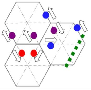
The cellular automata are models that discretize the space time and define automata in each point (cell) of the network that act in function of what their neighbors do (automata because they have a defined form of reacting). An example is a hexagonal structure:
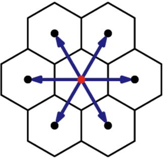
Model D2Q7 (two dimensions and 7 elements per cell - 6 sides and 1 center)
In the case that it is applied to a particulate gas, each node may or may not contain (states 0 and 1) a particle that can only have velocities with the directions that links between cells.
In the simulation with models like cellular automata there are two phases:
- cell acts on the others
- cell processes actions of the environment
In the special case of modeling a gas the first step corresponds to streaming while the second to collision (collision).
The mathematical description is performed by the particle distribution function
| $f_i(\vec{x},t)=w_if(\vec{x},\vec{v}_i,t)$ |
ID:(8494, 0)
D2Q9 Models (2 dimensions, 9 points)
Image
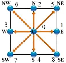
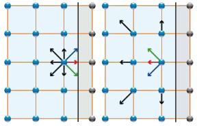
El modelo D2Q9 es un modelo bidimensional (D2) en que se se conecta el nodo (punto central) en nodos a lo largo de los ejes cartesianos\\n\\nen el origen\\n\\n
$\vec{e}_0=(0,0)$
\\n\\nen las esquinas\\n\\n
$\vec{e}_1=(1,0)$
(E),\\n
$\vec{e}_2=(0,1)$
(N), \\n
$\vec{e}_3=(-1,0)$
(W) y \\n
$\vec{e}_4=(0,-1)$
(S)\\n\\ny en las diagonales\\n\\n
$\vec{e}_5=(1,1)$
(NE), \\n
$\vec{e}_6=(-1,1)$
(SE), \\n
$\vec{e}_7=(-1,-1)$
(SW) y \\n
$\vec{e}_8=(1,-1)$
(NW)
lo que se representa en la siguiente gráfica:
ID:(8496, 0)
D3Q15 Models (3 dimensions, 15 points)
Note
The D3Q15 model is a two-dimensional model (D3) in which the node (central point) is connected in nodes along Cartesian axes\\n\\n
$(1,0,0), (-1,0,0), (0,1,0), (0,-1,0), (0,0,1) (0,0,-1)$
\\n\\nand in the corners of the bucket\\n\\n
$(1,0,1), (-1,0,1), (0,1,1) , (0,-1,1), (1,0,-1), (-1,0,-1), (0,1,-1) , (0,-1,-1)$
which is represented in the following graph:
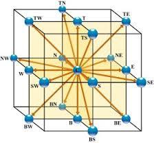
It is easy to build models of type D3Q19 (including side edge halves) or D3Q27 (all possible points).
ID:(8497, 0)
Streaming
Quote
En la etapa de steraming (flujo) se transportan las partículas de una celda según la dirección de la velocidad que tengan hacia el nodo correspondiente:
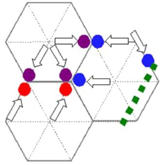
\\n\\nEn el caso del streaming se re calculan las funciones distribución en el sentido de que se re calculan sus componentes:\\n\\n
$f_i(\vec{x}+\vec{e}_i\delta t,t+\delta t)=f_i(\vec{x},t)$
En este punto también se incluye el efecto de los bordes que en el caso estático reflejan la velocidad (rebote) y en el caso que se estén moviendo la modifican.
ID:(8498, 0)
Collision
Exercise
En la etapa de colisiones se reasignan partículas de una dirección de velocidad a otra:
\\n\\nPara ello es necesario modelar la colisión que finalmente depende de la distribución misma y del tipo de interacción que exista. El resultado es que la nueva función distribución será:\\n\\n
$f_i(\vec{x},t+\delta t)=f_i(\vec{x},t)+C(f)$
ID:(8495, 0)
Borde simple
Equation
El borde mas simple es una pared paralela a la red misma de modo que las partículas pueden rebotar en forma simple:
\\n\\nEn estos casos la función distribución se deja fácilmente calcular simplemente invirtiendo la velocidad en la distribución en la posición simétrica al punto de rebote:\\n\\n
$f(\vec{x},e_i,t+\delta t)=f(\vec{x},-e_i,t)$
ID:(8501, 0)
Rebound in walls orthogonal to the network
Script
If the collision does not occur at the point of the network, but at a distance
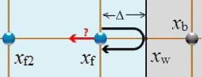
\\n\\nthen the function must consider the offset by weighting the contributions\\n\\n
$f_i(x_f,t+\delta t)=\displaystyle\frac{(1-\Delta)f_{-i}(x_f,t)+\Delta(f_{-i}(x_b,t)+f_{-i}(x_{f2},t)}{1+\Delta}$
ID:(8499, 0)
Rebound on walls with inclination
Variable
If the wall shows an inclination with respect to the network it must be modeled in a more complex form:
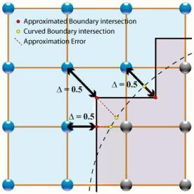
More general edge
First, an approximate boundary must be defined to allow the necessary edge equations to be established. Then they must be applied in the process of steraming.
ID:(8500, 0)
Rebote en paredes con Angulo
Audio
Si la pare se encuentra en movimiento a una velocidad $\vec{U}$ debe considerarse que puede incrementar o frenar a las partículas. En general se tendrá que\\n\\n
$f_i(\vec{e}_i,t+\delta t)=f_{-i}(\vec{e}_i)+G(\vec{e}_i,\vec{U})+G(-\vec{e}_i,-\vec{U})$
\\n\\nque se puede simplificar a \\n\\n
$f_i(e_i,t+\delta t)=f_{-i}(e_i)+\displaystyle\frac{6}{c^2}(\omega_im\vec{U}\cdot\vec{e}_i)$
ID:(8502, 0)
Estructuras y Automatas
Description
Variables
Calculations
Calculations
Equations
Examples
The cellular automata are models that discretize the space time and define automata in each point (cell) of the network that act in function of what their neighbors do (automata because they have a defined form of reacting). An example is a hexagonal structure:
Model D2Q7 (two dimensions and 7 elements per cell - 6 sides and 1 center)
In the case that it is applied to a particulate gas, each node may or may not contain (states 0 and 1) a particle that can only have velocities with the directions that links between cells.
In the simulation with models like cellular automata there are two phases:
- cell acts on the others
- cell processes actions of the environment
In the special case of modeling a gas the first step corresponds to streaming while the second to collision (collision).
The mathematical description is performed by the particle distribution function
| $f_i(\vec{x},t)=w_if(\vec{x},\vec{v}_i,t)$ |
(ID 8494)
El modelo D2Q9 es un modelo bidimensional (D2) en que se se conecta el nodo (punto central) en nodos a lo largo de los ejes cartesianos\\n\\nen el origen\\n\\n
$\vec{e}_0=(0,0)$
\\n\\nen las esquinas\\n\\n
$\vec{e}_1=(1,0)$
(E),\\n
$\vec{e}_2=(0,1)$
(N), \\n
$\vec{e}_3=(-1,0)$
(W) y \\n
$\vec{e}_4=(0,-1)$
(S)\\n\\ny en las diagonales\\n\\n
$\vec{e}_5=(1,1)$
(NE), \\n
$\vec{e}_6=(-1,1)$
(SE), \\n
$\vec{e}_7=(-1,-1)$
(SW) y \\n
$\vec{e}_8=(1,-1)$
(NW)
lo que se representa en la siguiente gr fica:
(ID 8496)
El modelo D2Q9 la distribuci n en equilibrio se describe mediante la ecuaci n
| $f_i^{eq}=\rho\omega_i\left[1+3\vec{e}_i\cdot\vec{u}+\displaystyle\frac{9}{2}(\vec{e}_i\cdot\vec{u})^2-\displaystyle\frac{3}{2}\mid\vec{u}|^2\right]$ |
\\n\\nen donde los pesos de la probabilidad son\\n\\n
$\omega_0=\displaystyle\frac{4}{9}$
\\n\\n
$\omega_1=\omega_2=\omega_3=\omega_4=\displaystyle\frac{1}{9}$
\\n\\n
$\omega_5=\omega_6=\omega_7=\omega_8=\displaystyle\frac{1}{36}$
(ID 8705)
El modelo D2Q9 la distribuci n se recalcula por efecto de las colisiones mediante
| $f_i^{new}=f_i^{old}+\displaystyle\frac{1}{\tau}(f_i^{eq}-f_i^{old})$ |
(ID 8706)
The D3Q15 model is a two-dimensional model (D3) in which the node (central point) is connected in nodes along Cartesian axes\\n\\n
$(1,0,0), (-1,0,0), (0,1,0), (0,-1,0), (0,0,1) (0,0,-1)$
\\n\\nand in the corners of the bucket\\n\\n
$(1,0,1), (-1,0,1), (0,1,1) , (0,-1,1), (1,0,-1), (-1,0,-1), (0,1,-1) , (0,-1,-1)$
which is represented in the following graph:
It is easy to build models of type D3Q19 (including side edge halves) or D3Q27 (all possible points).
(ID 8497)
En la etapa de steraming (flujo) se transportan las part culas de una celda seg n la direcci n de la velocidad que tengan hacia el nodo correspondiente:
\\n\\nEn el caso del streaming se re calculan las funciones distribuci n en el sentido de que se re calculan sus componentes:\\n\\n
$f_i(\vec{x}+\vec{e}_i\delta t,t+\delta t)=f_i(\vec{x},t)$
En este punto tambi n se incluye el efecto de los bordes que en el caso est tico reflejan la velocidad (rebote) y en el caso que se est n moviendo la modifican.
(ID 8498)
En la etapa de colisiones se reasignan part culas de una direcci n de velocidad a otra:
\\n\\nPara ello es necesario modelar la colisi n que finalmente depende de la distribuci n misma y del tipo de interacci n que exista. El resultado es que la nueva funci n distribuci n ser :\\n\\n
$f_i(\vec{x},t+\delta t)=f_i(\vec{x},t)+C(f)$
(ID 8495)
El borde mas simple es una pared paralela a la red misma de modo que las part culas pueden rebotar en forma simple:
\\n\\nEn estos casos la funci n distribuci n se deja f cilmente calcular simplemente invirtiendo la velocidad en la distribuci n en la posici n sim trica al punto de rebote:\\n\\n
$f(\vec{x},e_i,t+\delta t)=f(\vec{x},-e_i,t)$
(ID 8501)
If the collision does not occur at the point of the network, but at a distance
\\n\\nthen the function must consider the offset by weighting the contributions\\n\\n
$f_i(x_f,t+\delta t)=\displaystyle\frac{(1-\Delta)f_{-i}(x_f,t)+\Delta(f_{-i}(x_b,t)+f_{-i}(x_{f2},t)}{1+\Delta}$
(ID 8499)
If the wall shows an inclination with respect to the network it must be modeled in a more complex form:
More general edge
First, an approximate boundary must be defined to allow the necessary edge equations to be established. Then they must be applied in the process of steraming.
(ID 8500)
Si la pare se encuentra en movimiento a una velocidad $\vec{U}$ debe considerarse que puede incrementar o frenar a las part culas. En general se tendr que\\n\\n
$f_i(\vec{e}_i,t+\delta t)=f_{-i}(\vec{e}_i)+G(\vec{e}_i,\vec{U})+G(-\vec{e}_i,-\vec{U})$
\\n\\nque se puede simplificar a \\n\\n
$f_i(e_i,t+\delta t)=f_{-i}(e_i)+\displaystyle\frac{6}{c^2}(\omega_im\vec{U}\cdot\vec{e}_i)$
(ID 8502)
ID:(1035, 0)