
Examples of electric fields
Storyboard
Depending on the geometry of the distribution of charges, different electric fields are obtained.
ID:(1564, 0)
Gauss's law for a surface (1)
Equation
With Gauss's law
| $\displaystyle\int_S\vec{E}\cdot\hat{n}\,dS=\displaystyle\frac{Q}{\epsilon_0\epsilon}$ |
for the case that the field is normal and constant on only one surface we have
| $ E S = \displaystyle\frac{ Q }{ \epsilon\epsilon_0 }$ |
ID:(11456, 0)
Gauss's law for two surface (2)
Equation
With Gauss's law
| $\displaystyle\int_S\vec{E}\cdot\hat{n}\,dS=\displaystyle\frac{Q}{\epsilon_0\epsilon}$ |
for the case that the field is normal and constant on two surface we have
| $ E_1 S_1 + E_2 S_2 = \displaystyle\frac{ Q }{ \epsilon\epsilon_0 }$ |
ID:(11458, 0)
Gauss's law for three surface (3)
Equation
With Gauss's law
| $\displaystyle\int_S\vec{E}\cdot\hat{n}\,dS=\displaystyle\frac{Q}{\epsilon_0\epsilon}$ |
for the case that the field is normal and constant on three surface we have
| $ E_1 S_1 + E_2 S_2 + E_3 S_3 = \displaystyle\frac{ Q }{ \epsilon\epsilon_0 }$ |
ID:(11457, 0)
Conductor sphere with charge
Image
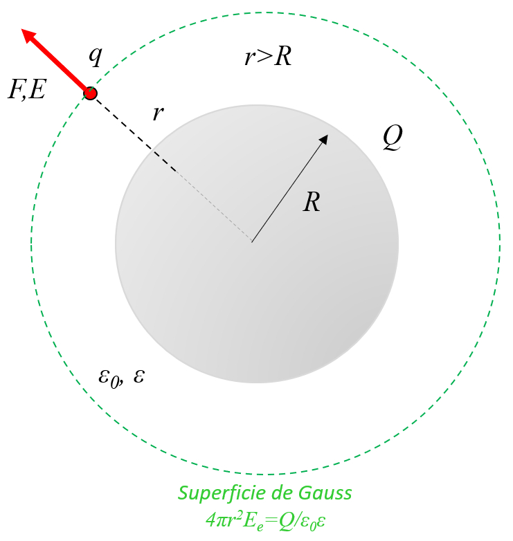
In a conducting sphere with charges, these are distributed on the surface and with it the field inside is null. Outside it behaves like a point charge that is in the center of the sphere:
ID:(11451, 0)
Surface of a sphere
Equation
La superficie de una esfera es con igual a
| $ S = 4 \pi r ^2$ |
ID:(4731, 0)
A single point charge
Equation
In the case of a spherical Gaussian surface, the field is constant, so it can be calculated by
| $ E S = \displaystyle\frac{ Q }{ \epsilon\epsilon_0 }$ |
with the surface of a sphere
| $ S = 4 \pi r ^2$ |
At a distance
| $ E_p =\displaystyle\frac{1}{4 \pi \epsilon_0 \epsilon }\displaystyle\frac{Q}{ r ^2}$ |
ID:(11442, 0)
Sphere with charge
Equation
Para el caso de una superficie gausseana esférica el campo es constante por lo que se puede calcular con charge $C$, constante de campo eléctrico $C^2/m^2N$, constante dieléctrica $-$, electric eield $V/m$ and surface $m^2$ mediante
| $ E S = \displaystyle\frac{ Q }{ \epsilon\epsilon_0 }$ |
con la superficie de una esfera con pi $rad$, radius of a circle $m$ and superficie $m^2$
| $ S = 4 \pi r ^2$ |
A una distancia
| $ E_f =\displaystyle\frac{1}{4 \pi \epsilon_0 \epsilon }\displaystyle\frac{Q}{ r ^2}\theta( r - R )$ |
ID:(11443, 0)
Loaded infinite wire or cylinder, in vacuum
Image
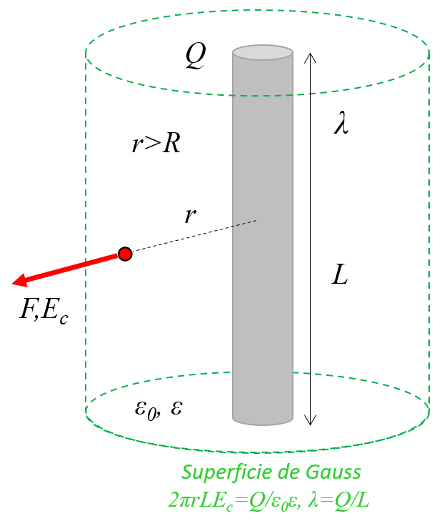
In a conductor wire or cylinder with charges, these are distributed throughout the object, behaving like a long chain of point loads aligned on the axis:
ID:(11452, 0)
Surface of a cylinder
Hypothesis
The surface of a cylinder of radius
ID:(10464, 0)
Linear load density
Equation
La densidad lineal de carga se calcula como la carga dividida por la carga que contiene el conductor lineal con es:
| $ \lambda = \displaystyle\frac{ Q }{ L }$ |
ID:(11459, 0)
Infinite wire
Equation
In the case of a cylindrica Gaussian surface, the field is constant, so it can be calculated by
| $ E S = \displaystyle\frac{ Q }{ \epsilon\epsilon_0 }$ |
with the surface of a cylinder
| $ S =2 \pi r h $ |
and the linear density
| $ \lambda = \displaystyle\frac{ Q }{ L }$ |
At a distance
| $ E_w =\displaystyle\frac{1}{2 \pi \epsilon_0 \epsilon }\displaystyle\frac{ \lambda }{ r }$ |
ID:(11444, 0)
Infinite conducting cylinder
Equation
Para el caso de una superficie gausseana cilíndrica el campo es constante por lo que se puede calcular con charge $C$, constante de campo eléctrico $C^2/m^2N$, constante dieléctrica $-$, electric eield $V/m$ and surface $m^2$ mediante
| $ E S = \displaystyle\frac{ Q }{ \epsilon\epsilon_0 }$ |
con la superficie de un cilindro con
| $ S =2 \pi r h $ |
y la densidad lineal con charge $C$, conductor length $m$ and linear charge density $C/m$
| $ \lambda = \displaystyle\frac{ Q }{ L }$ |
A una distancia
| $ E_c =\displaystyle\frac{1}{2 \pi \epsilon_0 \epsilon }\displaystyle\frac{ \lambda }{ r }\theta( r - R )$ |
ID:(11445, 0)
Insulating sphere with homogeneous charge
Image
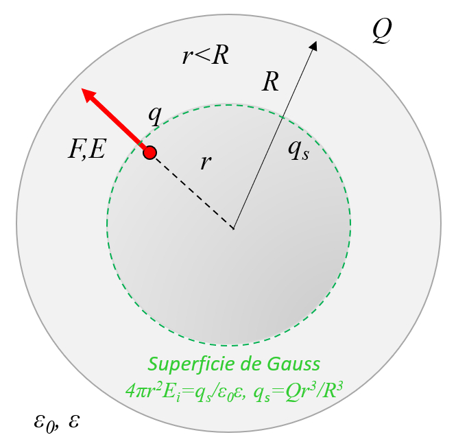
An insulating sphere in which charges have been homogeneously distributed, which cannot be moved because it is an insulating material, has an electric field that grows linearly inside and decreases with the inverse of the radius squared:
ID:(11450, 0)
Insulating sphere with full volume charge, exterior
Equation
Para el caso de una superficie gausseana esférica el campo es constante por lo que se puede calcular con charge $C$, constante de campo eléctrico $C^2/m^2N$, constante dieléctrica $-$, electric eield $V/m$ and surface $m^2$ mediante
| $ E S = \displaystyle\frac{ Q }{ \epsilon\epsilon_0 }$ |
con la superficie de una esfera con pi $rad$, radius of a circle $m$ and superficie $m^2$
| $ S = 4 \pi r ^2$ |
A una distancia
| $ E_e=\displaystyle\frac{1}{4 \pi \epsilon_0 \epsilon }\displaystyle\frac{ Q }{ r ^2 }$ |
ID:(11446, 0)
Charge fraction
Equation
In the case of a sphere of radius
| $ q =\displaystyle\frac{ r_i ^3 }{ R ^3 } Q $ |
ID:(11461, 0)
Insulating sphere with full volume charge, interior
Equation
Para el caso de una superficie gausseana esférica el campo es constante por lo que se puede calcular con charge $C$, constante de campo eléctrico $C^2/m^2N$, constante dieléctrica $-$, electric eield $V/m$ and surface $m^2$ mediante
| $ E S = \displaystyle\frac{ Q }{ \epsilon\epsilon_0 }$ |
con la superficie de una esfera con pi $rad$, radius of a circle $m$ and superficie $m^2$
| $ S = 4 \pi r ^2$ |
y la carga encerrada en la superficie gaussiana con charge $C$, encapsulated charge on Gauss surface $C$, internal radius $m$ and sphere radius $m$
| $ q =\displaystyle\frac{ r_i ^3 }{ R ^3 } Q $ |
A una distancia
| $ E_i =\displaystyle\frac{1}{4 \pi \epsilon_0 \epsilon }\displaystyle\frac{ Q r_i }{ R ^3 }$ |
ID:(11447, 0)
Infinite conductor plane with load
Image
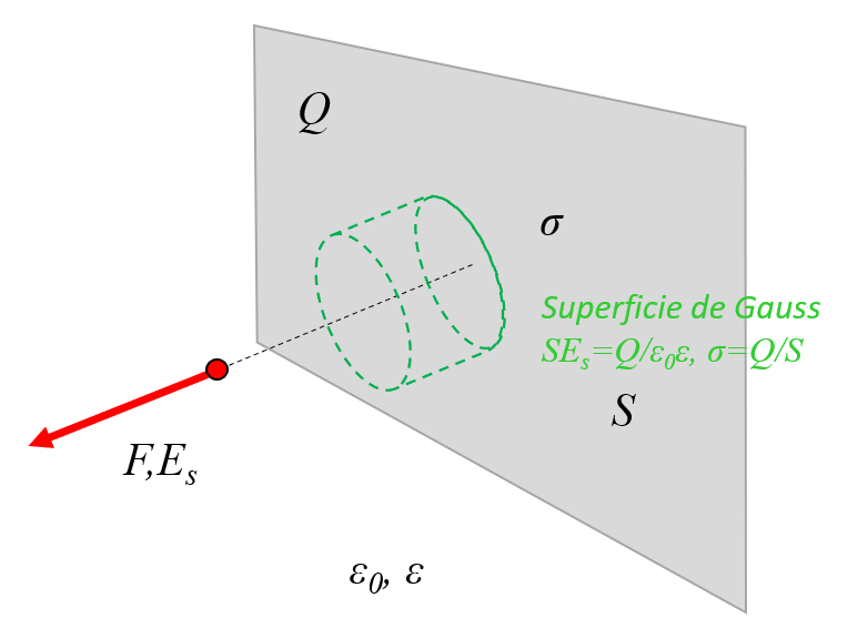
In a conducting plane, a Gaussian surface can be defined as a cylinder. The side walls are orthogonal to the field, so the only part that contributes are the surfaces parallel to the plane:
ID:(11453, 0)
Surface charge density
Equation
La densidad superficial de carga se calcula como la carga dividida por la superficie con es:
| $ \sigma = \displaystyle\frac{ Q }{ S }$ |
ID:(11460, 0)
Infinite plate
Equation
In the case of a flat Gaussian surface, the field is constant, so it can be calculated by
| $ E S = \displaystyle\frac{ Q }{ \epsilon\epsilon_0 }$ |
with the surface density of charges
| $ \sigma = \displaystyle\frac{ Q }{ S }$ |
The field for an infinite plate with a charge density per area
| $ E_s =\displaystyle\frac{ \sigma }{ 2 \epsilon_0 \epsilon }$ |
ID:(11448, 0)
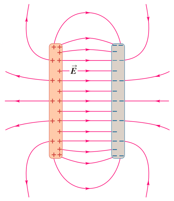
Two plates with opposite charges
Image
In the case of two plates with opposite charges there is a field of greater intensity between them. However, there is a minor field that can be described with field lines that emerge from one of the plates and return by giving an external turn to the opposite plate:
ID:(11454, 0)
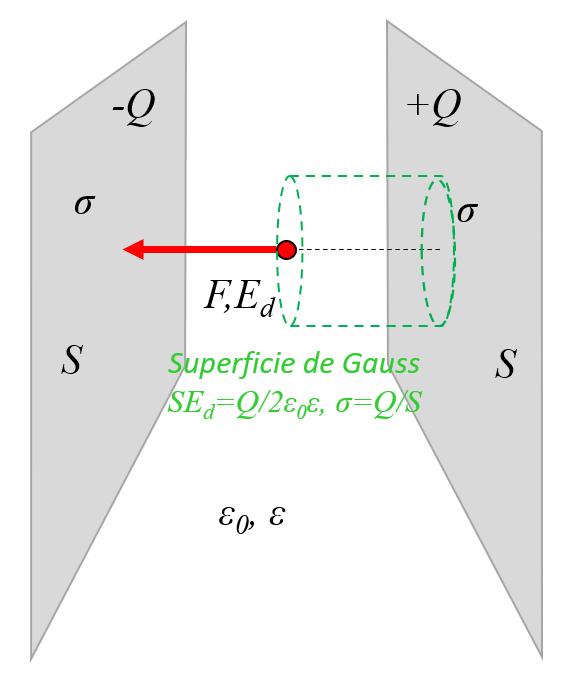
Simple model for two plates with opposite charges
Image
To be able to calculate the field between the two plates in a simple way, it can be assumed that the external field is compensated and that most of it is only between the plates:
ID:(11455, 0)
Two infinity plate with opposite plates
Equation
Para el caso de una superficie gausseana plana el campo es constante por lo que se puede con charge $C$, constante de campo eléctrico $C^2/m^2N$, constante dieléctrica $-$, electric eield $V/m$ and surface $m^2$ se calcular mediante
| $ E S = \displaystyle\frac{ Q }{ \epsilon\epsilon_0 }$ |
con la densidad de superficie de cargas con charge $C$, charge density by area $C/m^2$ and surface of the conductor $m^2$
| $ \sigma = \displaystyle\frac{ Q }{ S }$ |
El campo para de dos placa infinita con cargas opuestas con una densidad de carga por área
| $ E_d =\displaystyle\frac{ \sigma }{ \epsilon_0 \epsilon }$ |
ID:(11449, 0)
0
Video
Video: Examples of electric fields