
Random walk with variable pitch
Equation
The simplest case is that of a particular movimg along an axis that can impact some object, after which it will reverse its direction of advance.
If the probability of reaching a distance between
If this probability is proproposal to the probability itself
and get the probability function
| $p(x)dx = \displaystyle\frac{1}{\lambda}e^{-x/\lambda}dx$ |
We will call
ID:(9099, 0)
Normalization
Equation
If the distribution is integrated
| $p(x)dx = \displaystyle\frac{1}{\lambda}e^{-x/\lambda}dx$ |
over all possible distances
| $\displaystyle\int_0^{\infty}p(x)dx = \displaystyle\int_0^{\infty}\displaystyle\frac{1}{\lambda}e^{-x/\lambda}dx=1$ |
which means that the function is normalized. This is not surprising since the function
ID:(9251, 0)
Free path of a photon
Image
If the free path is given as a function of density, it can be compared between different materials. Being a function of the energy of the photon, it is obtained that the free path in bone and water are in the range 0 to 10MeV very similar:
image
If an estimate of the free path of the photon in water is desired, which shows a behavior very similar to that of tissue, it is sufficient to multiply the length in grams per square centimeter by the density, with which values between 0 and 30 cm are obtained.
ID:(9256, 0)
Free path of several particles
Image
If you compare the free paths for photons, neutrons, electrons and protons in water, observe differences in powers of ten:
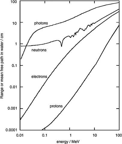
Free path of particles in water (ICRU report of 1970).
In this case the values are indicated in centimeters. For the range of up to 0.01 to 6 MeV the ranges (in cm) are
Particle | 0.01 MeV | 6 MeV
------------- |: ------------: |: ----------:
Photons | 0.198 | 41.7
Neutrons | 0.878 | 0.430
Electrons | 0.00032 | 0.211
Protons | - | 0.033
ID:(9257, 0)
Code structure (1)
Description
The structure of the simulation code must have three basic units:
- the definition of the distribution function (the arrangement that collects balls in the Galton table)
- the simulator of the advance of the particle that delivers the final position
- the unit that determines the class that must be increased in the distribution function (the unit that determines in which container of the receiver of balls this is deposited)
For the first point we must define an arrangement, which initially is set to zero, which is finally populated according to the position reached.
For the first step we must first define the range in which the ball falls, that is, a minimum value
If the arrangement we call it
```
// set distribution to cero
for(i = 0;i < num;i++){
p[i] = 0.0; // set to empty
}
```
Once they have been set to zero we must study the behavior of
```
Position calculation
```
Once you have obtained the position
With this value you can locate the container
```
cls = round((x-xmin)/Dx); // find position in array
p[cls]++; // increment array p in posicion cls on one
```
where the
ID:(9250, 0)
Path estimation
Equation
To simulate the path we must be able to randomly generate the free roads based on the distribution
| $p(x)dx = \displaystyle\frac{1}{\lambda}e^{-x/\lambda}dx$ |
To do this, it is enough to calculate the probability of achieving a path
and clear the way
| $x=-\lambda\ln(1-P)$ |
we obtain an equation that if we randomly generate a number between 0 and 1 we will obtain a path
With this you can define a function:
```
function exprob (len) {
var ran = Math.random ();
if (ran > 0) {
return -len*Math.log (1-ran);
} else {
return len;
}
}
```
in which we considered the generation of a number between 0 and 1 at random and we considered the possibility that the value is zero which would generate problems since the logarithm would be less infinite.
ID:(9255, 0)
Code structure (2)
Description
To calculate the final positions, you must:
- iterate over multiple particles (N)
- for each particle estimate the roads traveled
- add the roads alternating the directions of propagation
In this case it is assumed that in each collision the particle changes its propagation direction. In its beginning it always begins traveling increasing the distance which is defined as the positive direction (dir = 1). In each crash the dir sign is inverted (dir = -dir or dir = 1, this becomes dir = -1).
For the length of the step, the previously defined length generation function (exprob) is invoked, which is weighted with the address to obtain the new position with the previous position.
```
// particles (n de N)
for(n = 0;n < N;n++){
x = 0; // initial position
dir = 1; // initial direction
for(i = 0;i < sp;i++){
x = x + dir*exprob(len); // new position
dir = -dir; // change direction
}
// finish position calculation
// clasification of end position x in distribution p
}
```
ID:(9258, 0)
Simulador random walk variable pitch
Php
In order to obtain the distribution of the particulars according to the position, it is possible to perform an iteration in which
```
0. A starting position and direction is defined
1. It is displaced by a distance generated randomly as a function of the distance probability in a direction
2. the direction is reversed
3. continued in 1
```
If we assume that we expect a definite time and that the particle moves at constant speed, we can determine the position it has after a given time or after a definite total path.
ID:(9100, 0)