
The Otto Cycle
Storyboard 
The Otto cycle corresponds to an internal combustion engine in which heating occurs at a constant volume by turning on the mixture once the gas has been compressed.
ID:(1486, 0)
Mechanisms
Definition
The Otto cycle involves four main stages: intake, compression, power, and exhaust. During the intake phase, the engine draws in a mixture of fuel and air as the piston moves downwards. The mixture is then compressed as the piston moves upwards, which increases the temperature and pressure of the gas. At the top of the compression stroke, the spark plug ignites the compressed mixture, causing a rapid combustion known as the power stroke. This combustion pushes the piston back down, delivering power to the engine.
After the power stroke, the exhaust valve opens, and the piston moves back up to expel the spent gases from the combustion out of the cylinder, completing the cycle. The engine then repeats this cycle continuously during operation.
The efficiency of an Otto cycle engine depends on the degree of compression and the properties of the fuel used. Higher compression ratios typically lead to better efficiency but require higher octane fuel to prevent engine knocking. The Otto cycle is characterized by being a high-speed cycle with each stage clearly defined, contributing significantly to the overall efficiency and power output of engines that employ it.
ID:(15282, 0)
Carnot cycle
Image
Sadi Carnot introduced [1] the theoretical concept of the first machine design capable of generating mechanical work based on a heat gradient. This concept is realized through a process in the pressure-volume space where heat is added and extracted, as depicted in the image:
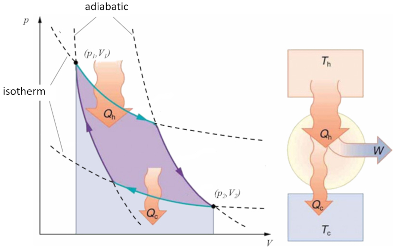
The area under curve the heat supplied ($Q_H$), spanning from 1 to 2, represents the energy input required to transition from state ($p_1, V_1$) to state ($p_2, V_2$). Conversely, the area under curve the absorbed heat ($Q_C$), going from 2 to 1, represents the energy extraction needed to return from state ($p_2, V_2$) back to state ($p_1, V_1$). The difference between these areas corresponds to the region enclosed by both curves and represents the effective work ($W$) that the system can perform.
Carnot also demonstrated that, in accordance with the second law of thermodynamics, the heat supplied ($Q_H$) cannot equal zero. This implies that no machine can convert all heat into work.
![]() [1] "Réflexions sur la puissance motrice du feu et sur les machines propres à développer cette puissance" (Reflections on the Motive Power of Fire and on Machines Fitted to Develop That Power), Sadi Carnot, Annales scientifiques de lÉ.N.S. 2e série, tome 1, p. 393-457 (1872)
[1] "Réflexions sur la puissance motrice du feu et sur les machines propres à développer cette puissance" (Reflections on the Motive Power of Fire and on Machines Fitted to Develop That Power), Sadi Carnot, Annales scientifiques de lÉ.N.S. 2e série, tome 1, p. 393-457 (1872)
ID:(11131, 0)
Otto cycle: Pressure-volume diagram
Note
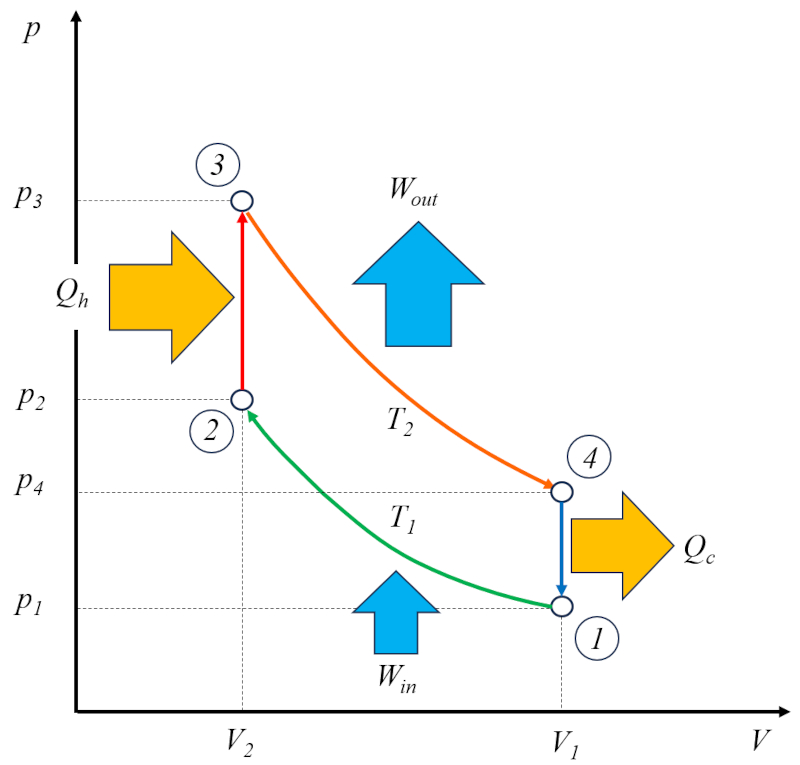
The Otto cycle [1] can be viewed as a technical solution based on the Carnot cycle. In this context, it consists of four stages:
• Stage 1 to 2: Adiabatic Compression $(p_1,V_1,T_1)\rightarrow(p_2,V_2,T_2)$,
• Stage 2 to 3: Heating $(p_2,V_2,T_2)\rightarrow(p_3,V_2,T_3)$,
• Stage 3 to 4: Adiabatic Expansion $(p_3,V_2,T_3)\rightarrow(p_4,V_1,T_4)$,
• Stage 4 to 1: Cooling $(p_4,V_1,T_4)\rightarrow(p_1,V_1,T_1)$
These stages are illustrated in the following diagram:

In the diagram, the energy flow is illustrated, where the heat supplied ($Q_H$) adds energy, raising the temperature from the temperature in state 2 ($T_2$) to the temperature in state 3 ($T_3$). It enters the system and performs ERROR:8165.1 units of work, while the counterpart the absorbed heat ($Q_C$) is absorbed, lowering the temperature from the temperature in state 4 ($T_4$) to the temperature in state 1 ($T_1$).
![]() [1] "Verbrennungsmotor" (Internal combustion engine), N. A. Otto, Kaiserlichen Patentamts, Patent 532, January 2, 1877
[1] "Verbrennungsmotor" (Internal combustion engine), N. A. Otto, Kaiserlichen Patentamts, Patent 532, January 2, 1877
Note: In 1862, Nikolaus Otto attempted to construct the internal combustion engine patented by Alphonse Beau de Rochas without success. He later modified it and succeeded in building a functional one in 1877, manufacturing 30,000 silent and highly reliable engines. He patented his design in 1877; however, the patent was later revoked due to the existence of Alphonse Beau de Rochas' patent, even though Rochas never managed to build his version. Since Otto was the first to make the engine work, his version is remembered today, labeling the process the "Otto Cycle."
ID:(11140, 0)
Technical Solution
Quote
The Otto engine operates in two cycles: the actual Otto cycle, which consists of the following phases:
• Phase 1 to 2: Adiabatic compression
• Phase 2 to 3: Heating
• Phase 3 to 4: Adiabatic expansion
• Phase 4 to 1: Cooling
In addition, it has a cycle for emptying the burnt gases and filling with a fresh mixture.
For this reason, it is referred to as a two-stroke engine. The emptying and filling phase can be accomplished using a compensating mass or through a second cylinder that operates out of phase.
The efficiency the efficiency ($\eta$) of the engine can be estimated using the otto compressibility factor ($r$) and the adiabatic index ($\kappa$) with the following equation:
| $ \eta = 1-\displaystyle\frac{1}{ r ^{ \kappa -1}}$ |
ID:(11142, 0)
Efficiency as a function of temperatures
Exercise
The absorbed heat ($Q_C$) is related to the heat capacity at constant volume ($C_V$), the temperature in state 4 ($T_4$), and the temperature in state 1 ($T_1$) according to the following equation:
| $ Q_C = C_V ( T_4 - T_1 )$ |
And the heat supplied ($Q_H$) is related to the heat capacity at constant volume ($C_V$), the temperature in state 3 ($T_3$), and the temperature in state 2 ($T_2$) through the equation:
| $ Q_H = C_V ( T_3 - T_2 )$ |
Therefore, in the equation for the efficiency ($\eta$) represented by:
| $ \eta = 1-\displaystyle\frac{ Q_C }{ Q_H } $ |
We have the following relationship:
| $ \eta =1-\displaystyle\frac{ T_4 - T_1 }{ T_3 - T_2 }$ |
ID:(15749, 0)
Efficiency depending on the compressibility factor
Equation
The efficiency ($\eta$), in terms of the temperature in state 1 ($T_1$), the temperature in state 2 ($T_2$), the temperature in state 3 ($T_3$), and the temperature in state 4 ($T_4$), is calculated using the equation:
| $ \eta =1-\displaystyle\frac{ T_4 - T_1 }{ T_3 - T_2 }$ |
In the case of adiabatic expansion, it is described using the adiabatic index ($\kappa$), the expanded volume ($V_1$), and the compressed volume ($V_2$) with the relationship:
| $ T_4 V_1 ^{ \kappa - 1} = T_3 V_2 ^{ \kappa - 1}$ |
And adiabatic compression is represented by the relationship:
| $ T_1 V_1 ^{ \kappa - 1} = T_2 V_2 ^{ \kappa - 1}$ |
If we subtract the second equation from the first, we obtain:
$(T_4 - T_1)V_1^{\kappa-1} = (T_3 - T_2)V_2^{\kappa-1}$
Which leads to the relationship:
$\left(\displaystyle\frac{V_1}{V_2}\right)^{\kappa-1} = \displaystyle\frac{T_3 - T_2}{T_4 - T_1}$
This, in turn, leads to the definition of the otto compressibility factor ($r$) with the equation:
| $ r =\displaystyle\frac{ V_1 }{ V_2 }$ |
With all these components, the efficiency of a process using the Otto cycle can be calculated as:
| $ \eta = 1-\displaystyle\frac{1}{ r ^{ \kappa -1}}$ |
ID:(15750, 0)
The Otto Cycle
Storyboard
The Otto cycle corresponds to an internal combustion engine in which heating occurs at a constant volume by turning on the mixture once the gas has been compressed.
Variables
Calculations
Calculations
Equations
Continuing the analogy to the ERROR:5219,0 for liquids and solids with the heat capacity ($C$) and the mass ($M$):
there is also a specific heat of gases at constant volume ($c_V$) for heating at constant volume with the heat capacity at constant volume ($C_V$):
When the absorbed heat ($Q_C$) is removed, the temperature of the gas increases from $T_1$ to $T_4$ in an isobaric process (at constant pressure). This implies that we can use the relationship for ERROR:8085 with the heat capacity at constant volume ($C_V$) and the variación de Temperature ($\Delta T$), which is expressed by the equation:
This leads us to the values of the temperature in state 1 ($T_1$) and the temperature in state 4 ($T_4$) using the formula:
When supplying the heat supplied ($Q_H$), the temperature of the gas increases from $T_2$ to $T_3$ in an isochoric process (at constant volume). This implies that we can utilize the relationship for ERROR:8085 with the heat capacity at constant volume ($C_V$) and the variación de Temperature ($\Delta T$), expressed by the equation:
This results in the temperature in state 2 ($T_2$) and the temperature in state 3 ($T_3$) as follows:
In an adiabatic expansion, the gas satisfies the relationship involving the volume in state i ($V_i$), the volume in state f ($V_f$), the temperature in initial state ($T_i$), and the temperature in final state ($T_f$):
In this case, from the initial point 3 to point 4. This means that during the adiabatic expansion, the state of the gas changes from the compressed volume ($V_2$) and the temperature in state 3 ($T_3$) to the expanded volume ($V_1$) and the temperature in state 4 ($T_4$) according to:
Given that in an adiabatic expansion, the gas satisfies the relationship with the volume in state i ($V_i$), the volume in state f ($V_f$), the temperature in initial state ($T_i$), and the temperature in final state ($T_f$):
In this case, from the initial point 1 to point 2. This means that during the adiabatic compression, the state of the gas changes from the expanded volume ($V_1$) and the temperature in state 1 ($T_1$) to the compressed volume ($V_2$) and the temperature in state 2 ($T_2$) as follows:
The absorbed heat ($Q_C$) is related to the heat capacity at constant volume ($C_V$), the temperature in state 4 ($T_4$), and the temperature in state 1 ($T_1$) according to the following equation:
And the heat supplied ($Q_H$) is related to the heat capacity at constant volume ($C_V$), the temperature in state 3 ($T_3$), and the temperature in state 2 ($T_2$) through the equation:
Therefore, in the equation for the efficiency ($\eta$) represented by:
We have the following relationship:
Adiabatic expansion is described using the variables the adiabatic index ($\kappa$), the temperature in state 4 ($T_4$), the temperature in state 3 ($T_3$), the expanded volume ($V_1$), and the compressed volume ($V_2$) through the relationship
While adiabatic compression is represented by the temperature in state 1 ($T_1$) and the temperature in state 2 ($T_2$) through the relationship
By subtracting the second equation from the first, we obtain
$(T_4 - T_1)V_1^{\kappa-1} = (T_3 - T_2)V_2^{\kappa-1}$
Which leads us to the relationship
$\left(\displaystyle\frac{V_1}{V_2}\right)^{\kappa-1} = \displaystyle\frac{T_3 - T_2}{T_4 - T_1}$
And this allows us to define the otto compressibility factor ($r$) as follows:
The efficiency ($\eta$), in terms of the temperature in state 1 ($T_1$), the temperature in state 2 ($T_2$), the temperature in state 3 ($T_3$), and the temperature in state 4 ($T_4$), is calculated using the equation:
In the case of adiabatic expansion, it is described using the adiabatic index ($\kappa$), the expanded volume ($V_1$), and the compressed volume ($V_2$) with the relationship:
And adiabatic compression is represented by the relationship:
If we subtract the second equation from the first, we obtain:
$(T_4 - T_1)V_1^{\kappa-1} = (T_3 - T_2)V_2^{\kappa-1}$
Which leads to the relationship:
$\left(\displaystyle\frac{V_1}{V_2}\right)^{\kappa-1} = \displaystyle\frac{T_3 - T_2}{T_4 - T_1}$
This, in turn, leads to the definition of the otto compressibility factor ($r$) with the equation:
With all these components, the efficiency of a process using the Otto cycle can be calculated as:
Examples
The Otto cycle involves four main stages: intake, compression, power, and exhaust. During the intake phase, the engine draws in a mixture of fuel and air as the piston moves downwards. The mixture is then compressed as the piston moves upwards, which increases the temperature and pressure of the gas. At the top of the compression stroke, the spark plug ignites the compressed mixture, causing a rapid combustion known as the power stroke. This combustion pushes the piston back down, delivering power to the engine.
After the power stroke, the exhaust valve opens, and the piston moves back up to expel the spent gases from the combustion out of the cylinder, completing the cycle. The engine then repeats this cycle continuously during operation.
The efficiency of an Otto cycle engine depends on the degree of compression and the properties of the fuel used. Higher compression ratios typically lead to better efficiency but require higher octane fuel to prevent engine knocking. The Otto cycle is characterized by being a high-speed cycle with each stage clearly defined, contributing significantly to the overall efficiency and power output of engines that employ it.
Sadi Carnot introduced [1] the theoretical concept of the first machine design capable of generating mechanical work based on a heat gradient. This concept is realized through a process in the pressure-volume space where heat is added and extracted, as depicted in the image:
The area under curve the heat supplied ($Q_H$), spanning from 1 to 2, represents the energy input required to transition from state ($p_1, V_1$) to state ($p_2, V_2$). Conversely, the area under curve the absorbed heat ($Q_C$), going from 2 to 1, represents the energy extraction needed to return from state ($p_2, V_2$) back to state ($p_1, V_1$). The difference between these areas corresponds to the region enclosed by both curves and represents the effective work ($W$) that the system can perform.
Carnot also demonstrated that, in accordance with the second law of thermodynamics, the heat supplied ($Q_H$) cannot equal zero. This implies that no machine can convert all heat into work.
![]() [1] "R flexions sur la puissance motrice du feu et sur les machines propres d velopper cette puissance" (Reflections on the Motive Power of Fire and on Machines Fitted to Develop That Power), Sadi Carnot, Annales scientifiques de l .N.S. 2e s rie, tome 1, p. 393-457 (1872)
[1] "R flexions sur la puissance motrice du feu et sur les machines propres d velopper cette puissance" (Reflections on the Motive Power of Fire and on Machines Fitted to Develop That Power), Sadi Carnot, Annales scientifiques de l .N.S. 2e s rie, tome 1, p. 393-457 (1872)
The Otto cycle [1] can be viewed as a technical solution based on the Carnot cycle. In this context, it consists of four stages:
• Stage 1 to 2: Adiabatic Compression $(p_1,V_1,T_1)\rightarrow(p_2,V_2,T_2)$,
• Stage 2 to 3: Heating $(p_2,V_2,T_2)\rightarrow(p_3,V_2,T_3)$,
• Stage 3 to 4: Adiabatic Expansion $(p_3,V_2,T_3)\rightarrow(p_4,V_1,T_4)$,
• Stage 4 to 1: Cooling $(p_4,V_1,T_4)\rightarrow(p_1,V_1,T_1)$
These stages are illustrated in the following diagram:
In the diagram, the energy flow is illustrated, where the heat supplied ($Q_H$) adds energy, raising the temperature from the temperature in state 2 ($T_2$) to the temperature in state 3 ($T_3$). It enters the system and performs ERROR:8165.1 units of work, while the counterpart the absorbed heat ($Q_C$) is absorbed, lowering the temperature from the temperature in state 4 ($T_4$) to the temperature in state 1 ($T_1$).
![]() [1] "Verbrennungsmotor" (Internal combustion engine), N. A. Otto, Kaiserlichen Patentamts, Patent 532, January 2, 1877
[1] "Verbrennungsmotor" (Internal combustion engine), N. A. Otto, Kaiserlichen Patentamts, Patent 532, January 2, 1877
Note: In 1862, Nikolaus Otto attempted to construct the internal combustion engine patented by Alphonse Beau de Rochas without success. He later modified it and succeeded in building a functional one in 1877, manufacturing 30,000 silent and highly reliable engines. He patented his design in 1877; however, the patent was later revoked due to the existence of Alphonse Beau de Rochas' patent, even though Rochas never managed to build his version. Since Otto was the first to make the engine work, his version is remembered today, labeling the process the "Otto Cycle."
The Otto engine operates in two cycles: the actual Otto cycle, which consists of the following phases:
• Phase 1 to 2: Adiabatic compression
• Phase 2 to 3: Heating
• Phase 3 to 4: Adiabatic expansion
• Phase 4 to 1: Cooling
In addition, it has a cycle for emptying the burnt gases and filling with a fresh mixture.
For this reason, it is referred to as a two-stroke engine. The emptying and filling phase can be accomplished using a compensating mass or through a second cylinder that operates out of phase.
The efficiency the efficiency ($\eta$) of the engine can be estimated using the otto compressibility factor ($r$) and the adiabatic index ($\kappa$) with the following equation:
The absorbed heat ($Q_C$) is related to the heat capacity at constant volume ($C_V$), the temperature in state 4 ($T_4$), and the temperature in state 1 ($T_1$) according to the following equation:
And the heat supplied ($Q_H$) is related to the heat capacity at constant volume ($C_V$), the temperature in state 3 ($T_3$), and the temperature in state 2 ($T_2$) through the equation:
Therefore, in the equation for the efficiency ($\eta$) represented by:
We have the following relationship:
The efficiency ($\eta$), in terms of the temperature in state 1 ($T_1$), the temperature in state 2 ($T_2$), the temperature in state 3 ($T_3$), and the temperature in state 4 ($T_4$), is calculated using the equation:
In the case of adiabatic expansion, it is described using the adiabatic index ($\kappa$), the expanded volume ($V_1$), and the compressed volume ($V_2$) with the relationship:
And adiabatic compression is represented by the relationship:
If we subtract the second equation from the first, we obtain:
$(T_4 - T_1)V_1^{\kappa-1} = (T_3 - T_2)V_2^{\kappa-1}$
Which leads to the relationship:
$\left(\displaystyle\frac{V_1}{V_2}\right)^{\kappa-1} = \displaystyle\frac{T_3 - T_2}{T_4 - T_1}$
This, in turn, leads to the definition of the otto compressibility factor ($r$) with the equation:
With all these components, the efficiency of a process using the Otto cycle can be calculated as:
In this case, from the initial point 1 to point 2. This means that during the adiabatic compression, the state of the gas changes from the expanded volume ($V_1$) and the temperature in state 1 ($T_1$) to the compressed volume ($V_2$) and the temperature in state 2 ($T_2$) as follows:
The heat supplied ($Q_H$) can be calculated from the heat capacity at constant volume ($C_V$), the temperature in state 2 ($T_2$) and the temperature in state 3 ($T_3$) using the formula:
In this case, from the initial point 3 to point 4. This means that during the adiabatic expansion, the state of the gas changes from the compressed volume ($V_2$) and the temperature in state 3 ($T_3$) to the expanded volume ($V_1$) and the temperature in state 4 ($T_4$) according to:
The absorbed heat ($Q_C$) can be calculated from the heat capacity at constant volume ($C_V$), the temperature in state 4 ($T_4$) and the temperature in state 1 ($T_1$) using the formula:
The efficiency ($\eta$) is a function of the temperature in state 1 ($T_1$), the temperature in state 2 ($T_2$), the temperature in state 3 ($T_3$) and the temperature in state 4 ($T_4$) is equal to :
The efficiency ($\eta$) is ultimately a function of the expanded volume ($V_1$) and the compressed volume ($V_2$), and in particular, of the otto compressibility factor ($r$):
The efficiency ($\eta$) can be calculated from the otto compressibility factor ($r$) and the adiabatic index ($\kappa$) in the case of the Otto cycle using:
The specific heat of gases at constant volume ($c_V$) is equal to the heat capacity at constant volume ($C_V$) divided by the mass ($M$):
ID:(1486, 0)