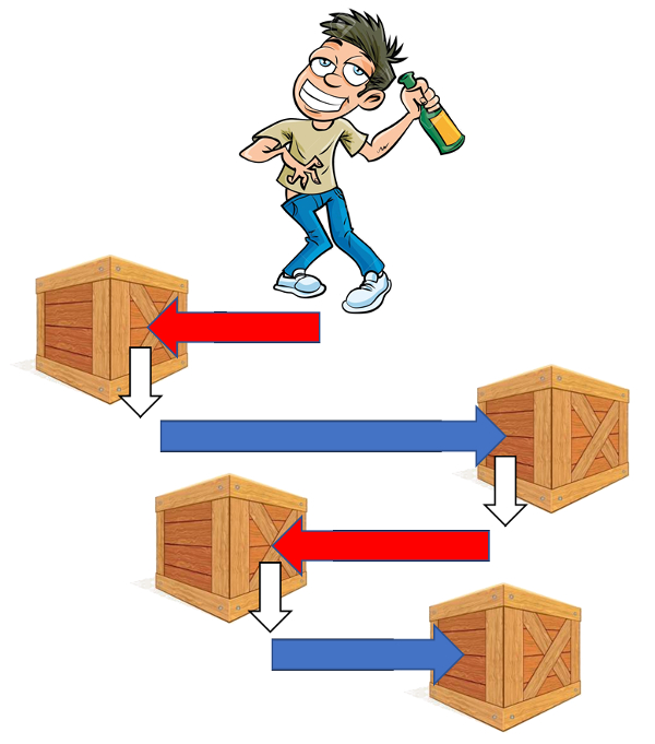
To explore the properties of Monte Carlo suppose that we want to simulate the behavior of a drunked.

He moves unidimensionally and can take steps to the right and to the left.

The distances traveled in each direction depend on the objects along the way. These are distributed randomly.

Each time he reaches an object, he reverses the direction in which he moves.

image

The simplest case is that of a particular movimg along an axis that can impact some object, after which it will reverse its direction of advance.

If the probability of reaching a distance between x and x+dx is P(x), the probability of impact will be equal to

P(x)-P(x+dx)\sim-\displaystyle\frac{dP}{dx}dx

If this probability is proproposal to the probability itself P, one has

\displaystyle\frac{dP}{dx}=-\displaystyle\frac{dx}{\lambda}P(x)

and get the probability function

equation

We will call \lambda the free path.

In order to obtain the distribution of the particulars according to the position, it is possible to perform an iteration in which

```

0. A starting position and direction is defined

1. It is displaced by a distance generated randomly as a function of the distance probability in a direction

2. the direction is reversed

3. continued in 1

```

If we assume that we expect a definite time and that the particle moves at constant speed, we can determine the position it has after a given time or after a definite total path.

Playing with the simulator we noticed that

```

1. It only makes sense to consider distributions of possible positions

2. The distribution is based on determining positions in discrete ranges

3. Ranges of smaller size require a greater number of iterations

```

The total effective section \sigma is related to the effective section that the particle offers to the incident beam and thus directly affects the free path. If it is multiplied by the concentration of the particles c it can be shown that the free path is

equation

with which it is possible to estimate the probability of impact with the total effective section:

Compton scattering occurs when a photon interacts with a charged particle, in particular with an electron. In the process the photon loses energy and deviates by putting the electron in motion:

image

Compton scattering occurs when a photon interacts with an electron by transferring the first energy to the second (inelastic interaction). The wavelength of the photon after the scattering can be calculated by

equation

where

equation=9146

Compton wave length and \theta the angle of deviation of the photon is.

In the case of Compton scattering, the differential effective section is according to Klein-Nishina

equation

where

equation=9112

is the Thomson total effective section and the

equation=9113

is the normalized energy.

If the differential effective section is taken according to Klein-Nishina

equation=9144

and integrates in the solid angle

equation=9147

the total effective section is obtained

equation

where

equation=9112

is the effective section of Thomson and the

equation=9113

is the normalized energy.

At the limit of small \epsilon\ll1 we have that the total section is

\sigma_{KN}\sim\sigma_T\left(1-2\epsilon+\displaystyle\frac{26}{5}\epsilon^2\ldots\right)

and in the limit \epsilon\gg 1 the total effective section is

\sigma_{KN}\sim\displaystyle\frac{3}{8}\displaystyle\frac{\sigma_T}{\epsilon}\left(\log(2\epsilon)+\displaystyle\frac{1}{2}\right)

The Klein-Nishina model can be studied in numerical form. This is shown

- the total effective section as a function of photon energy

- the differential section as a function of the angle for the minimum, medium and maximum energies defined

- what would be the total effective section in a one-dimensional system that gives according to the energy transmission or reflection