
Automatas Celulares
Definition 
The cellular automata are models that discretize the space time and define automata in each point (cell) of the network that act in function of what their neighbors do (automata because they have a defined form of reacting). An example is a hexagonal structure:
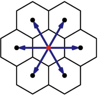
Model D2Q7 (two dimensions and 7 elements per cell - 6 sides and 1 center)
In the case that it is applied to a particulate gas, each node may or may not contain (states 0 and 1) a particle that can only have velocities with the directions that links between cells.
In the simulation with models like cellular automata there are two phases:
- cell acts on the others
- cell processes actions of the environment
In the special case of modeling a gas the first step corresponds to streaming while the second to collision (collision).
The mathematical description is performed by the particle distribution function
| $f_i(\vec{x},t)=w_if(\vec{x},\vec{v}_i,t)$ |
ID:(8494, 0)
D2Q9 Models (2 dimensions, 9 points)
Note
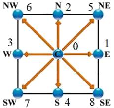
El modelo D2Q9 es un modelo bidimensional (D2) en que se se conecta el nodo (punto central) en nodos a lo largo de los ejes cartesianos\\n\\nen el origen\\n\\n
$\vec{e}_0=(0,0)$
\\n\\nen las esquinas\\n\\n
$\vec{e}_1=(1,0)$
(E),\\n
$\vec{e}_2=(0,1)$
(N), \\n
$\vec{e}_3=(-1,0)$
(W) y \\n
$\vec{e}_4=(0,-1)$
(S)\\n\\ny en las diagonales\\n\\n
$\vec{e}_5=(1,1)$
(NE), \\n
$\vec{e}_6=(-1,1)$
(SE), \\n
$\vec{e}_7=(-1,-1)$
(SW) y \\n
$\vec{e}_8=(1,-1)$
(NW)
lo que se representa en la siguiente gráfica:
ID:(8496, 0)
D3Q15 Models (3 dimensions, 15 points)
Quote
The D3Q15 model is a two-dimensional model (D3) in which the node (central point) is connected in nodes along Cartesian axes\\n\\n
$(1,0,0), (-1,0,0), (0,1,0), (0,-1,0), (0,0,1) (0,0,-1)$
\\n\\nand in the corners of the bucket\\n\\n
$(1,0,1), (-1,0,1), (0,1,1) , (0,-1,1), (1,0,-1), (-1,0,-1), (0,1,-1) , (0,-1,-1)$
which is represented in the following graph:
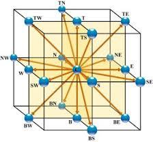
It is easy to build models of type D3Q19 (including side edge halves) or D3Q27 (all possible points).
ID:(8497, 0)
Discretization and Cell Structure of the LBM Approach
Storyboard
Variables
Calculations
Calculations
Equations
Examples
The cellular automata are models that discretize the space time and define automata in each point (cell) of the network that act in function of what their neighbors do (automata because they have a defined form of reacting). An example is a hexagonal structure:
Model D2Q7 (two dimensions and 7 elements per cell - 6 sides and 1 center)
In the case that it is applied to a particulate gas, each node may or may not contain (states 0 and 1) a particle that can only have velocities with the directions that links between cells.
In the simulation with models like cellular automata there are two phases:
- cell acts on the others
- cell processes actions of the environment
In the special case of modeling a gas the first step corresponds to streaming while the second to collision (collision).
The mathematical description is performed by the particle distribution function
In the case of the discretization in the LBM models we work not with functions of the speed if not with discrete components. In this way the
where
The dispersion is associated with the relaxation time
with
By discretizing we assume that the particles move with a mean velocity
El modelo D2Q9 es un modelo bidimensional (D2) en que se se conecta el nodo (punto central) en nodos a lo largo de los ejes cartesianos\\n\\nen el origen\\n\\n
$\vec{e}_0=(0,0)$
\\n\\nen las esquinas\\n\\n
$\vec{e}_1=(1,0)$
(E),\\n
$\vec{e}_2=(0,1)$
(N), \\n
$\vec{e}_3=(-1,0)$
(W) y \\n
$\vec{e}_4=(0,-1)$
(S)\\n\\ny en las diagonales\\n\\n
$\vec{e}_5=(1,1)$
(NE), \\n
$\vec{e}_6=(-1,1)$
(SE), \\n
$\vec{e}_7=(-1,-1)$
(SW) y \\n
$\vec{e}_8=(1,-1)$
(NW)
lo que se representa en la siguiente gr fica:
The D3Q15 model is a two-dimensional model (D3) in which the node (central point) is connected in nodes along Cartesian axes\\n\\n
$(1,0,0), (-1,0,0), (0,1,0), (0,-1,0), (0,0,1) (0,0,-1)$
\\n\\nand in the corners of the bucket\\n\\n
$(1,0,1), (-1,0,1), (0,1,1) , (0,-1,1), (1,0,-1), (-1,0,-1), (0,1,-1) , (0,-1,-1)$
which is represented in the following graph:
It is easy to build models of type D3Q19 (including side edge halves) or D3Q27 (all possible points).
ID:(1135, 0)