Constant acceleration, two stages
Storyboard 
In the case of accelerated motion in two stages, when transitioning from the first to the second acceleration, the final velocity of the first stage becomes the initial velocity of the second. The same applies to position, where the final position of the first stage equals the initial position of the second stage.
Unlike the two-speed model, this model does not exhibit discontinuity issues, except that acceleration can change abruptly, which is technically possible but often not very realistic.
ID:(1435, 0)
Constant acceleration, two stages
Storyboard
In the case of accelerated motion in two stages, when transitioning from the first to the second acceleration, the final velocity of the first stage becomes the initial velocity of the second. The same applies to position, where the final position of the first stage equals the initial position of the second stage. Unlike the two-speed model, this model does not exhibit discontinuity issues, except that acceleration can change abruptly, which is technically possible but often not very realistic.
Variables
Calculations
Calculations
Equations
In the case where the constant Acceleration ($a_0$) equals the mean Acceleration ($\bar{a}$), it will be equal to
Therefore, considering the speed Diference ($\Delta v$) as
and the time elapsed ($\Delta t$) as
the equation for the constant Acceleration ($a_0$)
can be written as
$a_0 = \bar{a} = \displaystyle\frac{\Delta v}{\Delta t} = \displaystyle\frac{v - v_0}{t - t_0}$
and by rearranging, we obtain
In the case of the constant Acceleration ($a_0$), the speed ($v$) as a function of the time ($t$) forms a straight line passing through the start Time ($t_0$) and the initial Speed ($v_0$), defined by the equation:
Since the distance traveled in a time ($\Delta s$) represents the area under the velocity-time curve, we can sum the contributions of the rectangle:
$v_0(t-t_0)$
and the triangle:
$\displaystyle\frac{1}{2}a_0(t-t_0)^2$
To obtain the distance traveled in a time ($\Delta s$) with the position ($s$) and the starting position ($s_0$), resulting in:
Therefore:
If we solve for the time ($t$) and the start Time ($t_0$) in the equation of the speed ($v$), which depends on the initial Speed ($v_0$) and the constant Acceleration ($a_0$):
we get:
$t - t_0= \displaystyle\frac{v - v_0}{a_0}$
And when we substitute this into the equation of the position ($s$) with the starting position ($s_0$):
we obtain an expression for the distance traveled as a function of velocity:
The definition of the mean Acceleration ($\bar{a}$) is considered as the relationship between the speed Diference ($\Delta v$) and the time elapsed ($\Delta t$). That is,
and
The relationship between both is defined as the centrifuge Acceleration ($a_c$)
within this time interval.
The definition of the mean Acceleration ($\bar{a}$) is considered as the relationship between the speed Diference ($\Delta v$) and the time elapsed ($\Delta t$). That is,
and
The relationship between both is defined as the centrifuge Acceleration ($a_c$)
within this time interval.
Examples
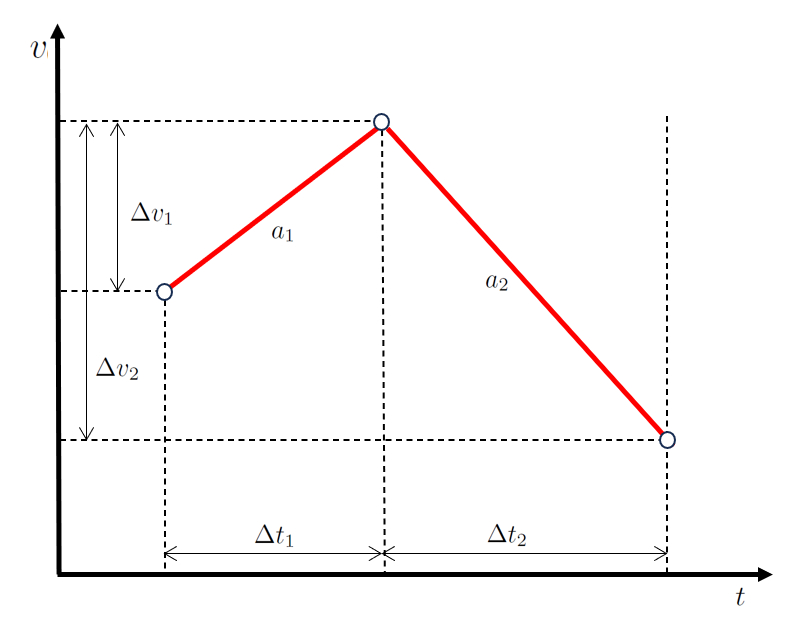
In a scenario of movement in two stages, first the object modifies its velocity by the speed difference in the first stage ($\Delta v_1$) during a time interval of ERROR:10242.1 with an acceleration of ERROR:10260.1.
Subsequently, in the second stage, it progresses by modifying its velocity by the speed difference in the second stage ($\Delta v_2$) during a time interval of the time spent in the second stage ($\Delta t_2$) with an acceleration of the acceleration during the second stage ($a_2$).
When represented graphically, we obtain a velocity and time diagram as shown below:
The key here is that the values the time spent in the first stage ($\Delta t_1$) and the time spent in the second stage ($\Delta t_2$) are sequential, just like the values the speed difference in the first stage ($\Delta v_1$) and the speed difference in the second stage ($\Delta v_2$).
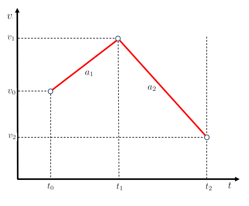
In the case of a two-stage movement, the first stage can be described by a function involving the points the start Time ($t_0$), the final time of first and start of second stage ($t_1$), the initial Speed ($v_0$), and the first stage speed ($v_1$), represented by a line with a slope of the acceleration during the first stage ($a_1$):
For the second stage, defined by the points the first stage speed ($v_1$), the second stage speed ($v_2$), the final time of first and start of second stage ($t_1$), and the second stage ending time ($t_2$), a second line with a slope of the acceleration during the second stage ($a_2$) is employed:
which is represented as:
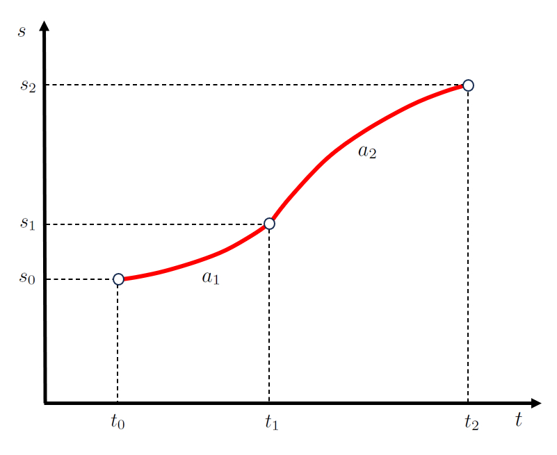
In the case of a two-stage movement, the position at which the first stage ends coincides with the position at the beginning of the second stage ($s_1$).
Similarly, the time at which the first stage ends coincides with the time at the beginning of the second stage ($t_1$).
Since the movement is defined by the acceleration experienced, the velocity attained at the end of the first stage must match the initial velocity of the second stage ($v_1$).
In the case of constant acceleration, in the first stage, the first final position and started second stage ($s_1$) depends on the starting position ($s_0$), the initial Speed ($v_0$), the acceleration during the first stage ($a_1$), the final time of first and start of second stage ($t_1$), and the start Time ($t_0$), as follows:
In the second stage, the second stage final position ($s_2$) depends on the first final position and started second stage ($s_1$), the first stage speed ($v_1$), the acceleration during the second stage ($a_2$), the final time of first and start of second stage ($t_1$), and the second stage ending time ($t_2$), as follows:
which is represented as:
If the movement involves two stages with different constant accelerations $a_1$ and $a_2$:
• It starts at time $t_0$ at position $s_0$ with velocity $v_0$.
• It ends at time $t_2$ at position $s_2$ with velocity $v_2$.
The key lies in the transition from one stage to the other:
• Velocities vary according to the accelerations but are equal at the transition point between stages ($v_1$).
• Positions vary according to velocity but are equal at the transition point between stages ($s_1$).
• Times are equal at the transition point between stages ($t_1$).
This is summarized in the following graphs:
The equations that fulfill these relationships give rise to the following model, which allows calculating any scenario:
Acceleration corresponds to the change in velocity per unit of time.
Therefore, it is necessary to define the speed Diference ($\Delta v$) in terms of the speed ($v$) and the initial Speed ($v_0$) as follows:
Acceleration corresponds to the change in velocity per unit of time.
Therefore, it is necessary to define the speed Diference ($\Delta v$) in terms of the speed ($v$) and the initial Speed ($v_0$) as follows:
To describe the motion of an object, we need to calculate the time elapsed ($\Delta t$). This magnitude is obtained by measuring the start Time ($t_0$) and the the time ($t$) of said motion. The duration is determined by subtracting the initial time from the final time:
To describe the motion of an object, we need to calculate the time elapsed ($\Delta t$). This magnitude is obtained by measuring the start Time ($t_0$) and the the time ($t$) of said motion. The duration is determined by subtracting the initial time from the final time:
The proportion in which the variation of velocity over time is defined as the mean Acceleration ($\bar{a}$). To measure it, it is necessary to observe the speed Diference ($\Delta v$) and the time elapsed ($\Delta t$).
One common method for measuring average acceleration involves using a stroboscopic lamp that illuminates the object at defined intervals. By taking a photograph, one can determine the distance traveled by the object in that time. By calculating two consecutive velocities, one can determine their variation and, with the time elapsed between the photos, the average acceleration.
The equation that describes average acceleration is as follows:
It is important to note that average acceleration is an estimation of actual acceleration.
The main problem is that if acceleration varies during the elapsed time, the value of the average acceleration may differ greatly from the mean acceleration
.
Therefore, the key is to
Determine acceleration over a sufficiently short period of time to minimize variation.
If the constant Acceleration ($a_0$), then the mean Acceleration ($\bar{a}$) is equal to the value of acceleration, that is,
In this case, the speed ($v$) as a function of the time ($t$) can be calculated by considering that it is associated with the difference between the speed ($v$) and the initial Speed ($v_0$), as well as the time ($t$) and the start Time ($t_0$).
This equation thus represents a straight line in velocity-time space.
In the case of ERROR:5297.1, the speed ($v$) varies linearly with the time ($t$), using the initial Speed ($v_0$) and the start Time ($t_0$):
Thus, the area under this line can be calculated, yielding the distance traveled in a time ($\Delta s$). Combining this with the starting position ($s_0$), we can calculate the position ($s$), resulting in:
This corresponds to the general form of a parabola.
In the case of constant acceleration, we can calculate the position ($s$) from the starting position ($s_0$), the initial Speed ($v_0$), the time ($t$), and the start Time ($t_0$) using the equation:
This allows us to determine the relationship between the distance covered during acceleration/deceleration and the change in velocity:
We can calculate the distance traveled in a time ($\Delta s$) from the starting position ($s_0$) and the position ($s$) using the following equation:
We can calculate the distance traveled in a time ($\Delta s$) from the starting position ($s_0$) and the position ($s$) using the following equation:
ID:(1435, 0)